MOLCAS manual:

Next: 10.4 High quality wave functions
Up: 10. Examples
Previous: 10.2 Geometry optimizations and Hessians.
Subsections
10.3 Computing a reaction path.
Chemists are familiarized with the description of a chemical
reaction as a continuous motion on certain path of the
potential energy hypersurfaces connecting reactants with
products. Those are considered minima in the hypersurface
while an intermediate state known as the transition state
would be a saddle point of higher energy. The height of the
energy barrier separating reactants from products relates
to the overall rate of reaction, the positions of the
minima along the reaction coordinate give the equilibrium
geometries of the species, and the relative energies relate
to the thermodynamics of the process. All this is known
as transition state theory.
The process to study a chemical reaction starts by obtaining
proper geometries for reactants and products, follows by finding the
position of the transition state, and finishes by computing
as accurately as possible the relative energies relating the
position of the species. To perform geometry optimizations
searching for true minima in the potential energy surfaces (PES)
is by now a well-established procedure (see section ![[*]](crossref.png) ).
An stationary point in the PES is characterized by having all the
first derivatives of the energy with respect to each one of the
independent coordinates equal to zero and the second derivatives
larger than zero. First-order saddle points, on the contrary, have their
second derivatives lower than zero for one coordinate,
that is, they are maxima along this coordinate. A
transition state is defined as a saddle point having only
one negative second derivative along the specific coordinate
known as the reaction coordinate. To simplify the treatment a special
set of coordinates known as normal coordinates is defined
in a way that the matrix of second derivatives is diagonal.
A transition state will have one negative value in the
diagonal of such a matrix. ).
An stationary point in the PES is characterized by having all the
first derivatives of the energy with respect to each one of the
independent coordinates equal to zero and the second derivatives
larger than zero. First-order saddle points, on the contrary, have their
second derivatives lower than zero for one coordinate,
that is, they are maxima along this coordinate. A
transition state is defined as a saddle point having only
one negative second derivative along the specific coordinate
known as the reaction coordinate. To simplify the treatment a special
set of coordinates known as normal coordinates is defined
in a way that the matrix of second derivatives is diagonal.
A transition state will have one negative value in the
diagonal of such a matrix.
Finally once the reactant, product and transition state geometries have been established one
could perform a Intrinsic Reaction Coordinate (IRC) analysis. This to find the energy profile
of the reaction and also to establish that the found transition state is connected to the
reactant and the product.
10.3.1 Studying a reaction
The localization of the transition state of a reaction is of importance
in both a qualitative and quantitative description of the reaction mechanism and
the thermodynamics of a reaction.
In the following example we will locate the
transition state of the proton transfer reaction between the two species
in Figs. and .
The example selected here is chosen
to demonstrate the steps needed to find a transition state. For that sake we have
limited our model to the SCF level of theory.
Figure 10.5:
Reactant
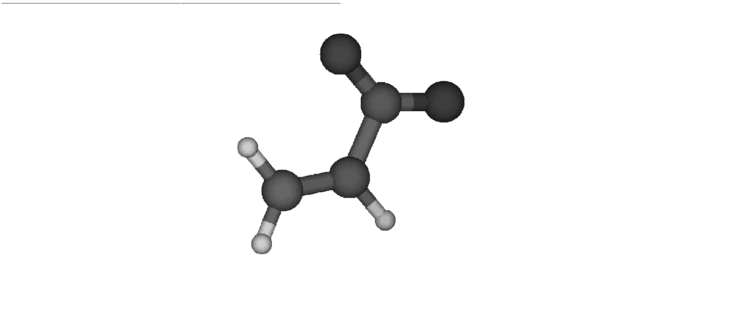 |
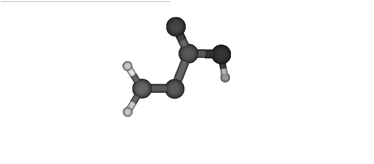
Figure 10.6:
Product
 |
The first step is to establish the two species in equilibrium. These calculations
would constitute standard geometry optimizations with the input for the reactant
>>> Do while <<<
&Seward
Basis set
C.cc-pVDZ....
C1 -1.9385577715 0.0976565175 0.4007212526
C2 -2.4151209200 -0.0592579424 2.8519334864
C3 0.7343463765 0.0088689871 -0.7477660837
End of Basis
Basis set
H.cc-pVDZ....
H1 -4.3244501026 0.0091320829 3.6086029352
H2 -0.8591520071 -0.2642180524 4.1663142585
H3 -3.4743702487 0.3026128386 -0.9501874771
End of Basis
Basis set
O.cc-pVDZ....
O1 0.7692102769 0.1847569555 -3.0700425345
O2 2.4916838932 -0.2232135341 0.7607580753
End of Basis
End of input
>>> IF ( ITER = 1 ) <<<
&SCF
Core
Charge = -1
>>> ENDIF <<<
&SCF &End
LUMORB
Charge = -1
&Slapaf
Iterations = 20
>>> EndDo <<<
resulting in the following convergence pattern
Energy Grad Grad Step Estimated Hessian Geom Hessian
Iter Energy Change Norm Max Element Max Element Final Energy Index Update Update
1 -265.09033194 0.00000000 0.091418 0.044965 nrc003 0.069275 nrc003 -265.09529138 0 RF(S) None
2 -265.09646330-0.00613136 0.020358 0.008890 nrc003 0.040393 nrc008 -265.09684474 0 RF(S) BFGS
3 -265.09693242-0.00046912 0.011611-0.005191 nrc001 0.079285 nrc016 -265.09709856 0 RF(S) BFGS
4 -265.09655626 0.00037616 0.020775-0.010792 nrc016-0.070551 nrc016 -265.09706324 0 RF(S) BFGS
5 -265.09706308-0.00050682 0.003309-0.001628 nrc003-0.010263 nrc017 -265.09707265 0 RF(S) BFGS
6 -265.09707056-0.00000747 0.000958-0.000450 nrc011 0.017307 nrc017 -265.09707924 0 RF(S) BFGS
7 -265.09706612 0.00000444 0.002451 0.001148 nrc003-0.011228 nrc018 -265.09706837 0 RF(S) BFGS
8 -265.09707550-0.00000938 0.000516 0.000220 nrc001-0.004017 nrc014 -265.09707591 0 RF(S) BFGS
9 -265.09707586-0.00000036 0.000286 0.000104 nrc001 0.002132 nrc017 -265.09707604 0 RF(S) BFGS
and for the product the input
>>> Do while <<<
&Seward
Basis set
C.cc-pVDZ....
C1 -2.0983667072 0.1000525724 0.5196668948
C2 -2.1177298783 -0.0920244467 3.0450747772
C3 0.5639781563 0.0024463770 -0.5245225314
End of Basis
Basis set
H.cc-pVDZ....
H1 -3.8870548756 -0.0558560582 4.1138131865
H2 -0.4133953535 -0.2946498869 4.2050068095
H3 -1.3495534119 0.3499572533 -3.3741881412
End of Basis
Basis set
O.cc-pVDZ....
O1 0.5100106099 0.2023808294 -3.0720173949
O2 2.5859515474 -0.2102046338 0.4795705925
End of Basis
End of input
>>> IF ( ITER = 1 ) <<<
&SCF
Core
Charge = -1
>>> ENDIF <<<
&SCF
LUMORB
Charge = -1
&Slapaf
Iterations = 20
>>> EndDo <<<
resulting in the following convergence pattern
Energy Grad Grad Step Estimated Hessian Geom Hessian
Iter Energy Change Norm Max Element Max Element Final Energy Index Update Update
1 -265.02789209 0.00000000 0.062885-0.035740 nrc006-0.060778 nrc006 -265.02939600 0 RF(S) None
2 -265.02988181-0.00198972 0.018235-0.011496 nrc006-0.023664 nrc006 -265.03004886 0 RF(S) BFGS
3 -265.03005329-0.00017148 0.001631-0.000978 nrc009-0.015100 nrc017 -265.03006082 0 RF(S) BFGS
4 -265.03004953 0.00000376 0.002464-0.000896 nrc014 0.013752 nrc017 -265.03006022 0 RF(S) BFGS
5 -265.03006818-0.00001865 0.001059 0.000453 nrc013-0.007550 nrc014 -265.03007064 0 RF(S) BFGS
6 -265.03006524 0.00000294 0.001800 0.000778 nrc014 0.006710 nrc014 -265.03007032 0 RF(S) BFGS
7 -265.03006989-0.00000465 0.000381 0.000190 nrc005 0.003078 nrc016 -265.03007014 0 RF(S) BFGS
8 -265.03006997-0.00000008 0.000129-0.000094 nrc016-0.001305 nrc017 -265.03007003 0 RF(S) BFGS
The computed reaction energy is estimated to about 42 kcal/mol at this level of theory.
To locate the transition state it is important to identify the reaction coordinate.
In our case here we note that the significant reaction coordinates are the bond distances between C1
and H3, and O1 and H3. In the location of the transition state we
will start from the geometry of the reactant for which the O1-H3 bond distance is
2.51 Ångström. We will conduct the search in a number of constrained geometry
optimizations in which we step by step reduce the O1-H3 distance towards the distance
in the product of 0.95 Ångström. The selected series is 2.0, 1.5, 1.3, and
1.0 Ångström.
To constraint the O1-H3 bond distance we modify the input to the
GATEWAY moduel by adding the following:
Constraint
R1 = Bond H3 O1
Value
R1 = 2.0 Angstrom
End of Constraint
The SLAPAF module's associated input looks like:
&Slapaf &End
Iterations
20
FindTS
PRFC
End of Input
This will correspond to the input for the first of the series of constraint
geometry optimization. However, note the keyword FindTS. This
keyword will make the SLAPAF module switch from a constrained geometry optimization
to a transition state geometry optimization if the updated geometrical
Hessian contains one negative eigenvalue. It is of course our hope that during the
series of constrained geometry optimizations that we will run into
this situation and find the transition state. The convergence pattern for the first
constrained optimization is
Energy Grad Grad Step Estimated Hessian Geom Hessian
Iter Energy Change Norm Max Element Max Element Final Energy Index Update Update
1 -265.09707600 0.00000000 0.965614 0.965614 Cns001 0.230366* nrc009 -265.07671229 0 MFRFS None
2 -265.08759913 0.00947687 0.216939 0.214768 Cns001 0.081441 nrc012 -265.08946379 0 MFRFS MSP
3 -265.08218288 0.00541624 0.014770 0.007032 nrc010 0.019690 nrc010 -265.08242668 0 MFRFS MSP
4 -265.08251826-0.00033537 0.003644-0.001560 nrc003 0.005075 nrc002 -265.08254163 0 MFRFS MSP
5 -265.08254834-0.00003008 0.001274-0.000907 nrc012 0.026237! nrc016 -265.08257455 0 MFRFS MSP
6 -265.08251413 0.00003421 0.003036-0.002420 nrc016-0.024325 nrc016 -265.08254699 0 MFRFS MSP
7 -265.08254682-0.00003269 0.000837-0.000426 nrc012 0.012351 nrc017 -265.08255083 0 MFRFS MSP
8 -265.08255298-0.00000616 0.000470 0.000238 nrc016-0.005376 nrc017 -265.08255421 0 MFRFS MSP
9 -265.08255337-0.00000038 0.000329-0.000154 nrc012-0.004581 nrc014 -265.08255409 0 MFRFS MSP
10 -265.08255418-0.00000081 0.000206-0.000148 nrc012-0.000886 nrc014 -265.08255425 0 MFRFS MSP
11 -265.08255430-0.00000013 0.000123-0.000097 nrc012-0.001131 nrc014 -265.08255436 0 MFRFS MSP
Here we note that the Hessian index is zero, i.e. the optimization is a constrained
geometry optimization. The final structure is used as the starting geometry for
the 2nd constrained optimization at 1.5 Ångström. This optimization did not find a negative
eigenvalue either. However, starting the 3rd constrained optimization from the final
structure of the 2nd constrained optimization resulted in the convergence pattern
Energy Grad Grad Step Estimated Hessian Geom Hessian
Iter Energy Change Norm Max Element Max Element Final Energy Index Update Update
1 -265.03250948 0.00000000 0.384120 0.377945 Cns001-0.209028* nrc007 -264.99837542 0 MFRFS None
2 -265.01103140 0.02147809 0.120709 0.116546 Cns001-0.135181 nrc007 -265.01209656 0 MFRFS MSP
3 -265.00341440 0.00761699 0.121043-0.055983 nrc005-0.212301* nrc007 -264.98788416 1 MFRFS MSP
4 -264.99451339 0.00890101 0.089986 0.045423 nrc007 0.123178* nrc002 -264.99582814 1 MFRFS MSP
5 -264.99707885-0.00256546 0.044095-0.015003 nrc009 0.159069* nrc015 -265.00090995 1 MFRFS MSP
6 -264.99892919-0.00185034 0.033489-0.013653 nrc015-0.124146 nrc015 -265.00050567 1 MFRFS MSP
7 -265.00031159-0.00138240 0.009416-0.004916 nrc018-0.156924 nrc018 -265.00070286 1 MFRFS MSP
8 -265.00019076 0.00012083 0.009057 0.005870 nrc018 0.081240 nrc018 -265.00049408 1 MFRFS MSP
9 -265.00049567-0.00030490 0.003380 0.001481 nrc011-0.070124 nrc015 -265.00056966 1 MFRFS MSP
10 -265.00030276 0.00019291 0.159266-0.159144 Cns001 0.114927! nrc015 -264.99874954 0 MFRFS MSP
11 -265.00098377-0.00068101 0.031621-0.008700 nrc005-0.101187 nrc007 -265.00046906 1 MFRFS MSP
12 -265.00050857 0.00047520 0.003360 0.001719 nrc015 0.012580 nrc015 -265.00052069 1 MFRFS MSP
13 -265.00052089-0.00001233 0.001243-0.000590 nrc017-0.006069 nrc017 -265.00052323 1 MFRFS MSP
14 -265.00052429-0.00000340 0.000753 0.000259 nrc011-0.002449 nrc018 -265.00052458 1 MFRFS MSP
15 -265.00052441-0.00000011 0.000442-0.000136 nrc007 0.003334 nrc018 -265.00052464 1 MFRFS MSP
16 -265.00052435 0.00000006 0.000397 0.000145 nrc017 0.001628 nrc010 -265.00052459 1 MFRFS MSP
Here a negative Hessian eigenvalue was found at iteration 3. At this point the optimization turn to a normal
quasi-Newton Raphson optimization without any constraints. We note that the procedure flips back to a constrained
optimization at iteration 10 but is finished as an optimization for a transition state.
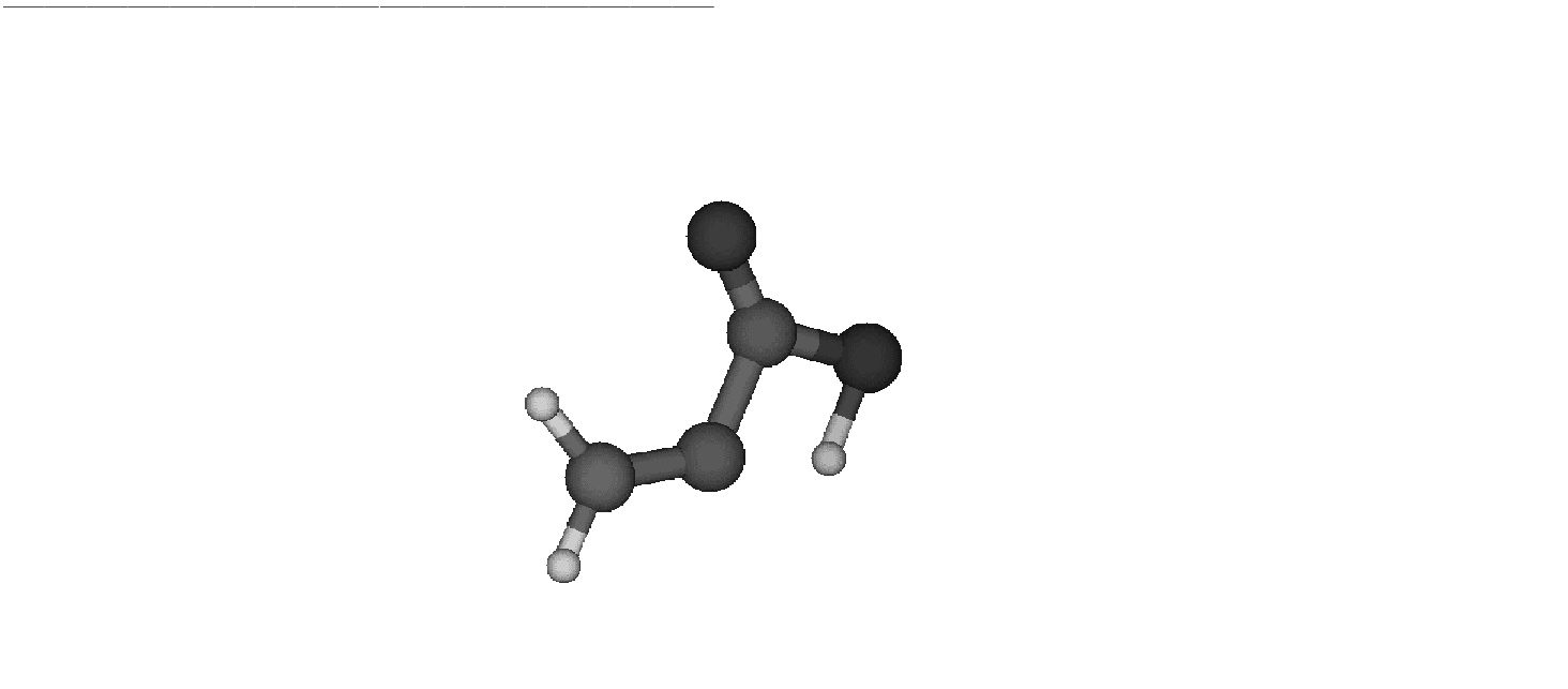
The predicted activation energy is estimated to 60.6 kcal/mol (excluding vibrational corrections).
The computed transition state
is depicted in Fig. .
Figure 10.7:
Transition state
 |
The remaining issue is if this is a true transition state. This issue can only be
resolved by doing a calculation of the analytical Hessian using the
MCKINLEY module (execution of the MCLR module is automatic). The corresponding input is
&Seward
Basis set
C.cc-pVDZ....
C1 -1.8937541206 0.0797525492 0.5330826031
C2 -2.3239194706 -0.0748842444 3.0012862573
C3 0.7556108398 -0.0065134659 -0.5801137465
End of Basis
Basis set
H.cc-pVDZ....
H1 -4.2196708766 -0.0106202053 3.8051971560
H2 -0.7745261239 -0.2775291936 4.3506967746
H3 -1.9256618348 0.2927045555 -2.1370156139
End of Basis
Basis set
O.cc-pVDZ....
O1 0.2162486684 0.2196587542 -2.9675781183
O2 2.8171388123 -0.2187115071 0.3719375423
End of Basis
End of input
&SCF
Charge = -1
&McKinley
Perturbation
Hessian
From the output of the MCLR code
***********************************
* *
* Harmonic frequencies in cm-1 *
* Intensities in km/mole *
* *
* No correction due to curvlinear *
* representations has been done *
* *
***********************************
Symmetry a
==============
1 2 3 4 5 6
Freq. i2027.40 i2.00 i0.07 0.05 0.07 2.02
...
...
7 8 9 10 11 12
Freq. 3.57 145.36 278.41 574.44 675.27 759.94
...
...
13 14 15 16 17 18
Freq. 927.78 943.60 1000.07 1225.34 1265.63 1442.57
...
...
19 20 21 22 23 24
Freq. 1517.91 1800.86 1878.11 2294.83 3198.94 3262.66
we can conclude that we have one imaginary eigenvalue (modes 2-7 corresponds to the translational
and rotational zero frequency modes) and that the structure found with this procedure indeed is a
transition state. A post calculation analysis of the vibrational modes using the MOLDEN package
confirm that the vibrational mode with the imaginary frequency is a mode which moves the proton from
the oxygen to the carbon.
A minimum energy path (MEP) is defined as the path defined by a sequence of geometries obtained by a
series of optimizations on a hypersphere. The series of constrained optimization starts from some
starting structure and the optimized structure at each step is taken as the start for the next step.
The constraint in these optimizations is the radius (in mass weighted coordinates) of the hyper sphere
with the origin defined by the starting geometry. If the starting structure is a transition state the
path is called an Intrinsic Reaction Coordinate (IRC) path. Since the transition structure (TS) has a negative
index of the Hessian we have two paths away from the TS. One leading us to the product(s) and one going to
the reactant(s). The IRC analysis is used to verify whether the TS is really connecting the expected
reactant(s) and product(s) and it is performed in forward and backward directions starting from the TS.
This analysis is obtained using the keyword IRC with the SLAPAF
specifying the number of points and, if different from the default value (0.10 au), the radius
of the hypersphere with the keywords nIRC and IRCStep, respectively.
The reaction vector can be found on RUNOLD or it can be specified explicitly (see keyword "REACtion vector").
In the latter case, the vector can be find at the end of the optimization job in the
"The Cartesian Reaction vector" section of the SLAPAF output.
A file named $Project.irc.molden (read by MOLDEN ) will be generated
in $WorkDir containing only those points belonging to the IRC.
Here an example for an IRC analysis with 20 points back and forth and with 0.05 au as step.
The reaction vector will be read on RUNOLD.
>>> EXPORT MOLCAS_MAXITER=500
>>> Do while <<<
...
&Slapaf &End
IRC
nIRC
20
IRCStep
0.05
Iterations
200
End of Input
>>> EndDo <<<
If the file RUNFILE is not available, the reaction vector must be specified in the
input.
>>> EXPORT MOLCAS_MAXITER=500
>>> Do while <<<
...
&Slapaf &End
IRC
nIRC
20
IRCStep
0.05
REACtion vector
0.140262 0.000000 0.179838
0.321829 0.000000 -0.375102
-0.006582 0.000000 -0.048402
-0.032042 -0.018981 -0.003859
-0.423466 0.000000 0.247525
Iterations
200
End of Input
>>> EndDo <<<
    
Next: 10.4 High quality wave functions
Up: 10. Examples
Previous: 10.2 Geometry optimizations and Hessians.
|