light grid and geometry viewer: lgv

Tutorial

Editing molecular structures with the lgv program.

The lgv program is used to manipulate molecular structures, build new molecules, and visualize orbitals, densities, and related properties. Here, we show how structures can be manipulated.

To open a coordinate file, use the command lgv Water.xyz. To create a new file, use the -n flag:  lgv -n Water.xyz. If no filename is specified, lgv  will open the first coordinate file it finds in the current directory.

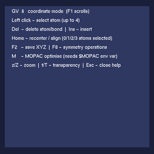
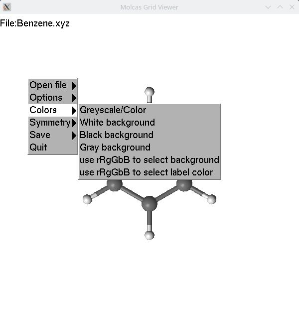
Some common hot keys are shown when the F1 key is pressed. Additional menus are available via right-click.

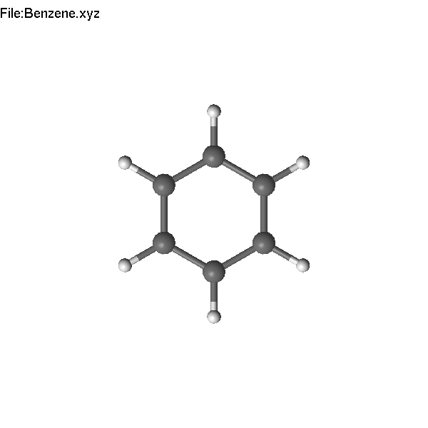
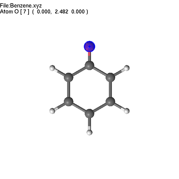
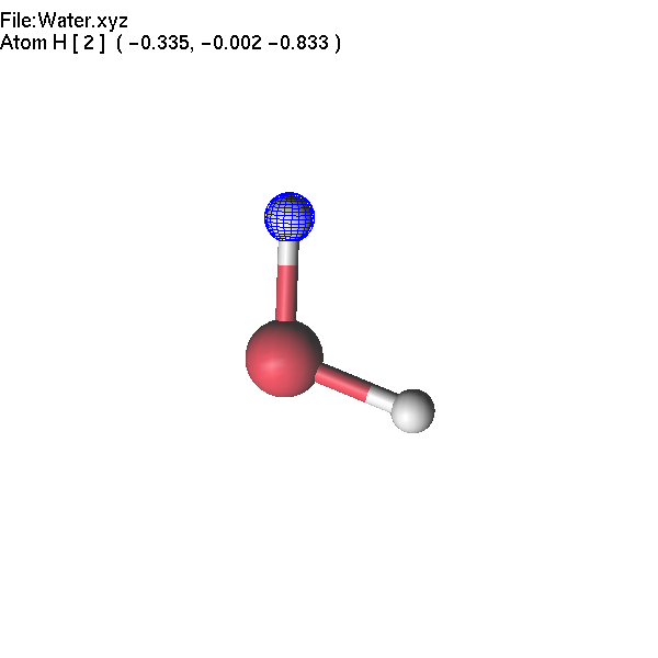
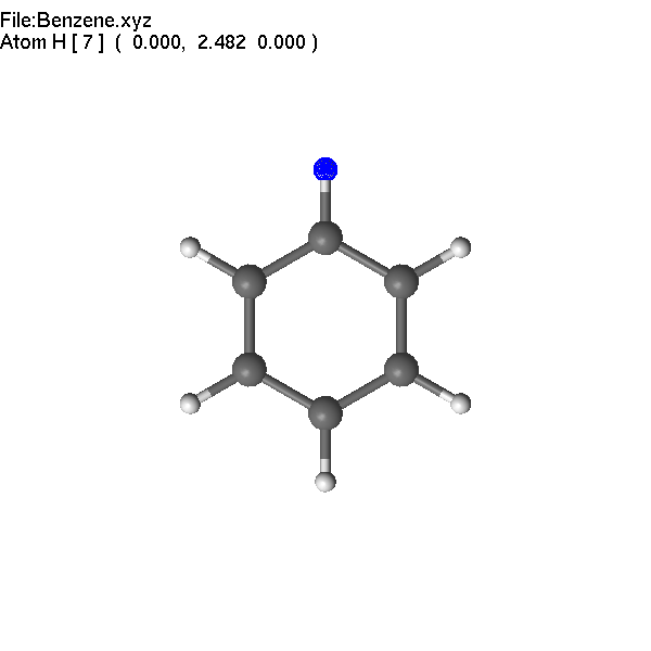
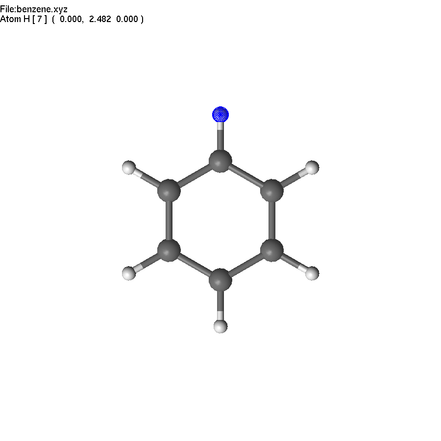
In order to modify coordinates, we have to select one, two, three or four atoms. Selection is made by clicking on an atom. The first selected atom is covered by a blue-colored net; the following selected atoms are covered by a magenta-colored net. The number of selected atoms determines the behavior of lgv. If only one atom is selected, operations apply to this atom. If two atoms are selected, operations apply to the bond connecting these atoms. If three atoms are selected, operations apply to the angle. Finally, four selected atoms define the dihedral angle. As a general rule, '+/-' changes the value of the selected object, PageUp/PageDown changes its property, and = (or F4) allows you to set the value.
To remove the selection, press the Space bar or click the middle mouse button. Pressing + or - will modify the value. For example, if a bond is selected and the user presses the '+' key, the bond length will increase, so the first selected atom will move away from the second atom.

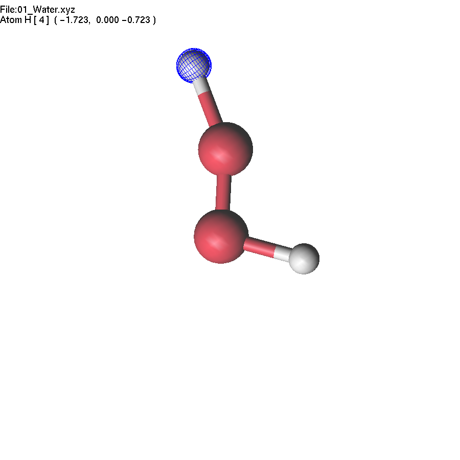
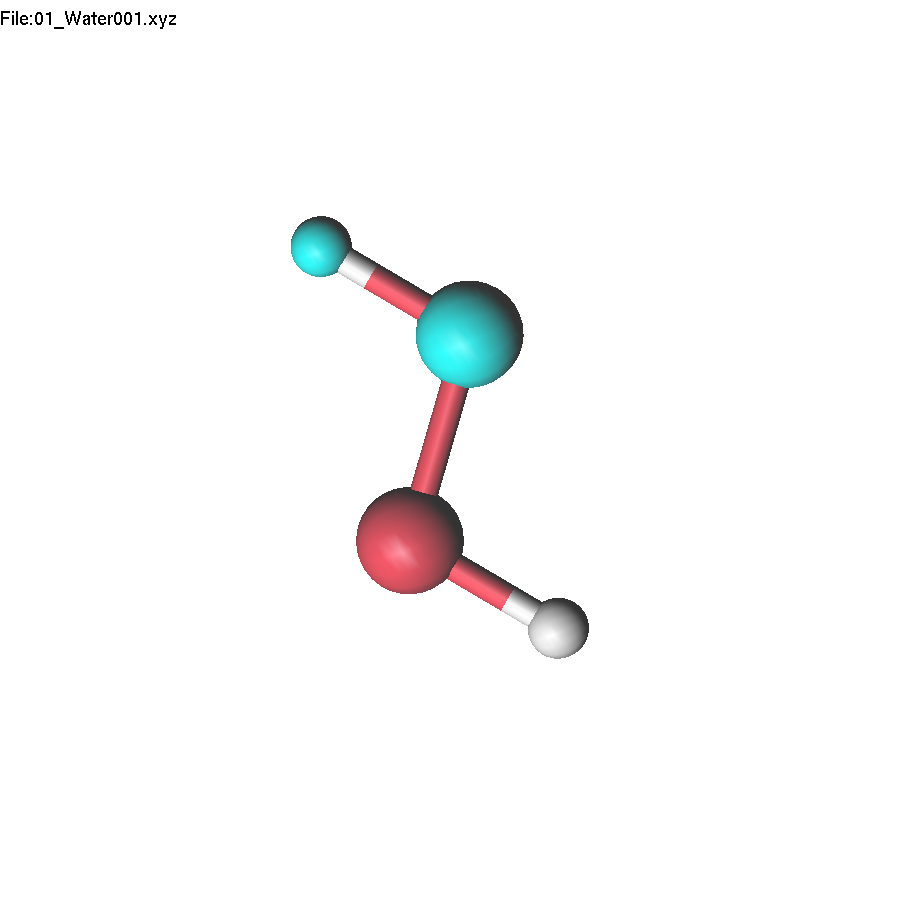
Example of selected atom:

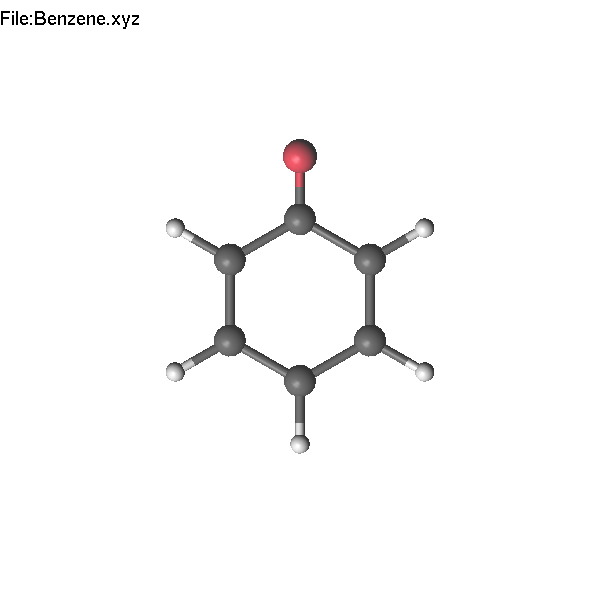
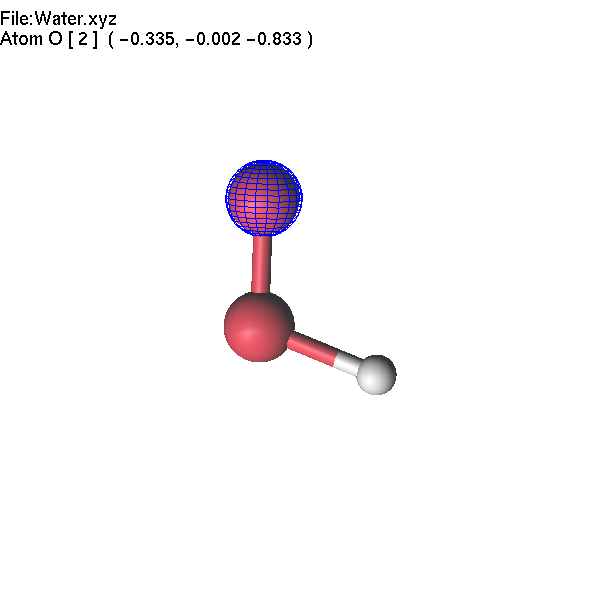
Pressing F4 (or =) and typing O (note that you do not need to focus into 'edit' window), we change the H atom to O.

It is also possible to use PgUp to change the atom name using the list of the most common elements.

The Backspace key can be used to undo modifications.

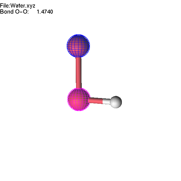
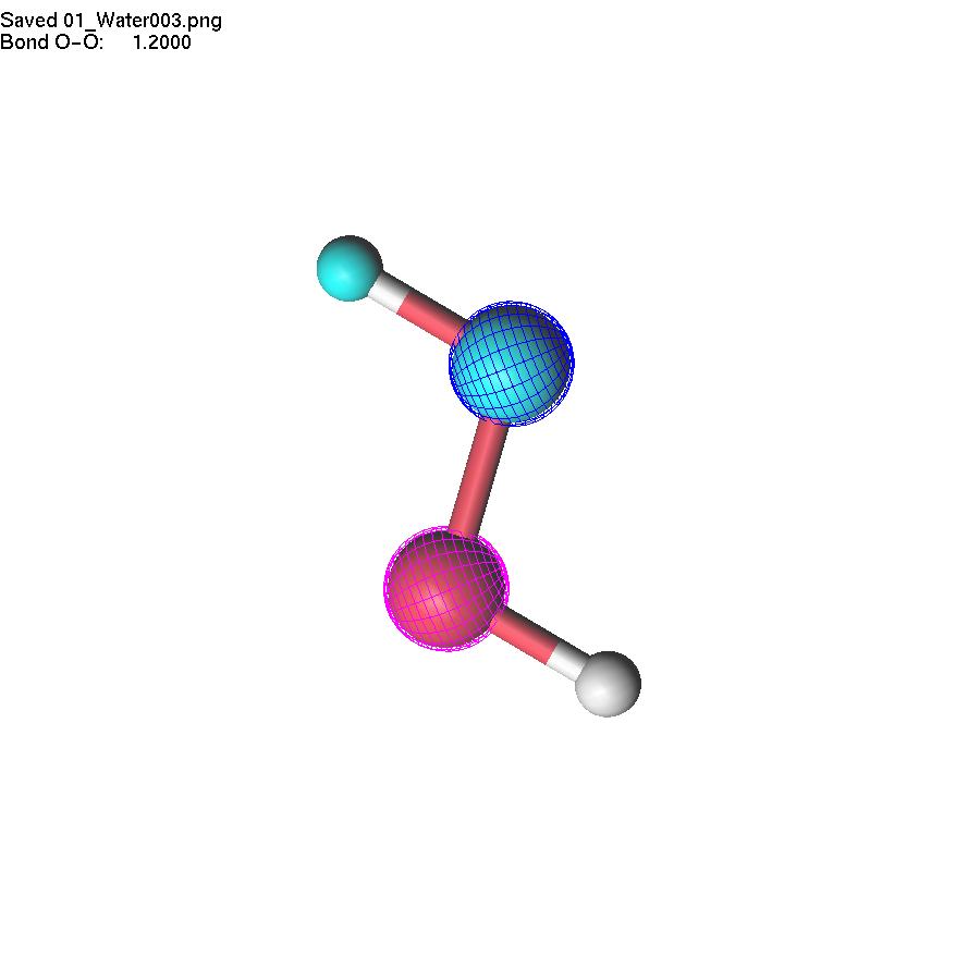
If two atoms are selected, the bond length can be modified using +/- or =/F4.

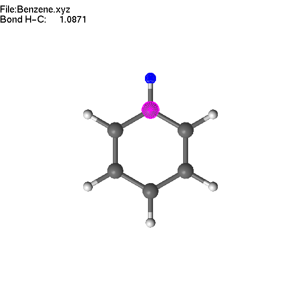
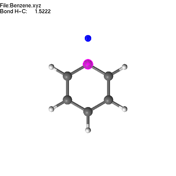
Note that the first atom (blue) moves during the operation.

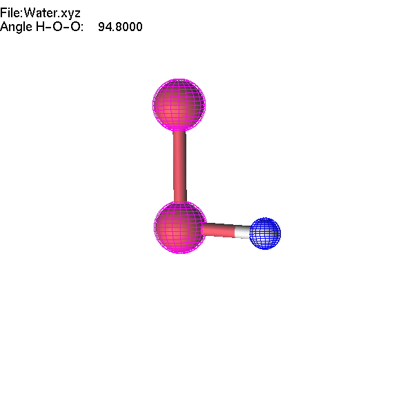
Similarly, if three atoms are selected, the angle value will be modified, and if four atoms are selected, the dihedral angle will be modified.

Pressing PageUp/PageDown modifies the 'property' of the selected object. If only one atom is selected - it will change element name, if a bond is selected, it changes the type of the bond (single, double, etc.), and if an angle is selected, it changes the angle to common values.

F2 key can be used to save the coordinate file. The file name is generated from the original name by adding a counter. Shift-F2 will overwrite the original file. These operations work for XYZ, Molden, and lus files.

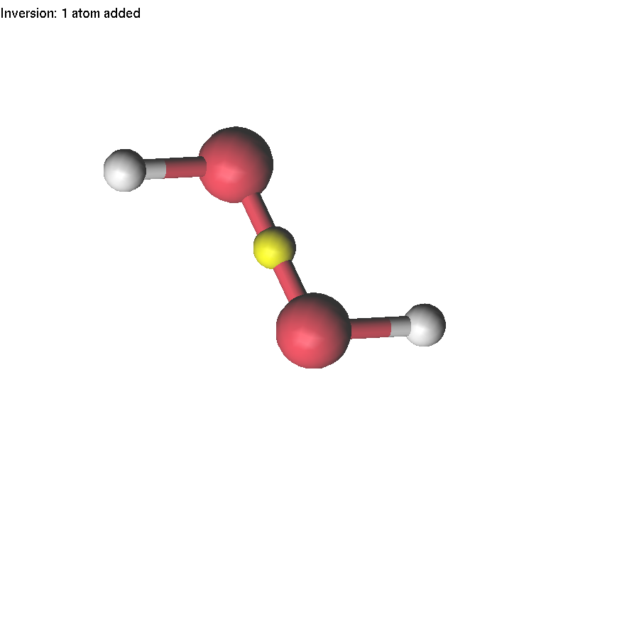
If one atom is selected, you can use the Delete or Insert key to delete it or insert a new atom. These operations are available for XYZ, Molden, and lus files. Let us make an H₂O₂ molecule starting from the Water.xyz file.

• select a H atom
• press PageUp until the atom becomes oxygen.

  

• alternatively, you can press F4 (or =) and type O (note that you do not need to position the mouse in the green input box)
• select another O atom
• press F4 (or =) and type 1.474 followed by Enter

  

• press the Space bar (or click the middle mouse button) to unselect the atoms.
• if you select three atoms, H-O-O, you can modify the angle
• press F4 and type 94.8 followed by Enter
• press the Space bar to unselect the atoms

• 

• now, make sure that you have only one oxygen selected (one without H), and press Insert (or I, if your keyboard does not have Insert button). The result: another H atom appears on the screen near the previously selected atom. The atom is already selected, so you can fix its position with respect to the other atoms.

  

• building a molecule by inserting atoms (or fragments) is difficult, because you need to fix all internal coordinates. An alternative way to edit the molecule is to use symmetry.
• select two Oxygen atoms
• press End to create a dummy atom in the middle of the bond

  

• select this dummy atom
• press F8 to apply inversion symmetry

  

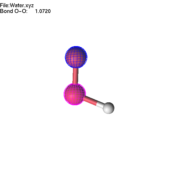
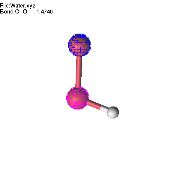
Now we will continue to edit the H₂O₂ molecule. If we select the O-O bond and change the interatomic distance, only one atom will move. If we want to move a group (O-H), we have to highlight this group first.

There are several ways to highlight (mark) a group of atoms. Probably the simplest way is to use the mouse. Press and hold the Shift key and drag the mouse. All atoms in this rectangular area will be highlighted. Another possibility is to hold the Shift key and click an atom with the mouse; this toggles the status of this atom. It is also possible to use the F7 key to make a selection. If no atom is selected, F7 highlights H atoms. If one atom is selected, F7 highlights its neighbours (atoms connected to this atom), and 'a' highlights all atoms of the same element.

To remove highlighting, press the Space bar or the middle mouse button.

Now, we can make operations with a group of atoms. Select two atoms: first the highlighted oxygen atom, then the non-highlighted one. Then press + until the highlighted fragment is far enough from the other oxygen atom that lgv no longer shows the bond. Note that the decision about which atoms are 'bonded' is based entirely on atomic radii (which can be adjusted).

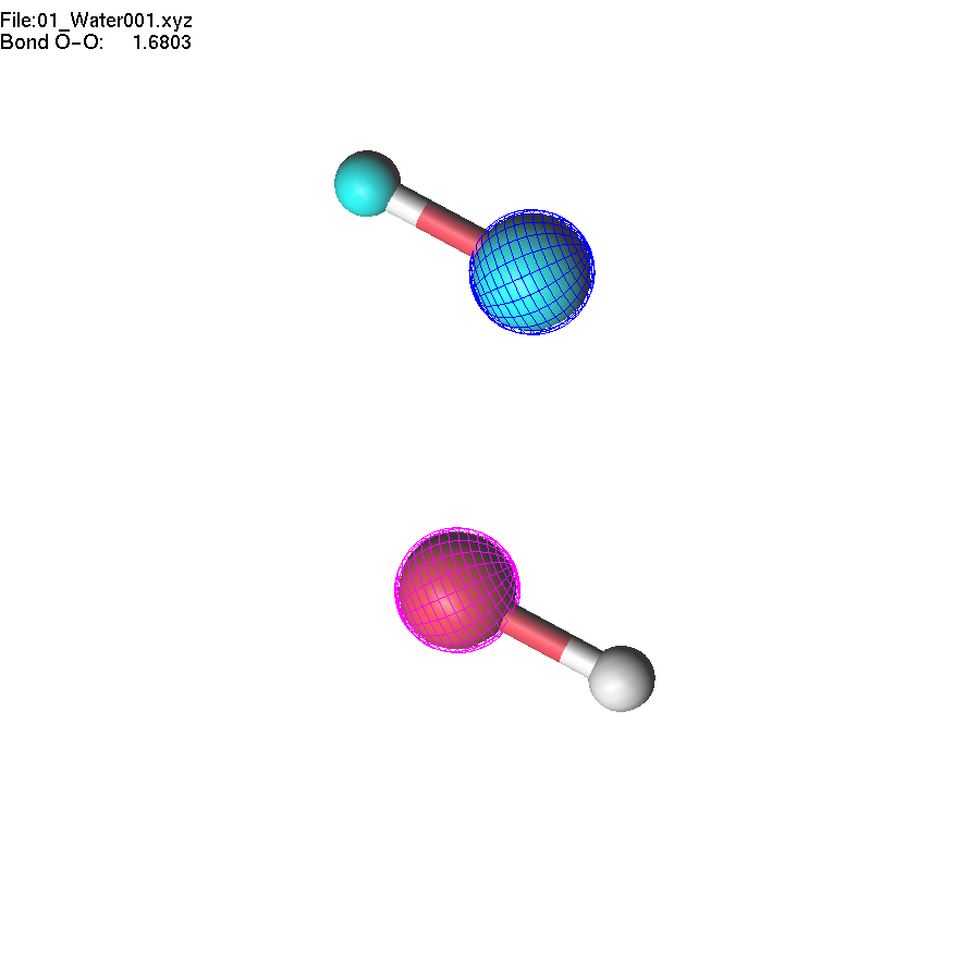
If you change the length of the O-O bond, the whole highlighted group will move accordingly. Note that unselection (Space key, or mouse middle click) will remove selection first, and the second use of the unselect button removes the highlighting of the group.

The modified value (of a bond length or an angle) is shown on the information line of the screen. Sometimes you may want to observe another value while modifying coordinates. To do this, select a bond or an angle and press the F6 key. Now you can make another selection and make modifications in the geometry. In this case, the originally selected value will be watched. Pressing Shift-F6 switches off watch mode.

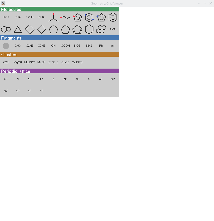
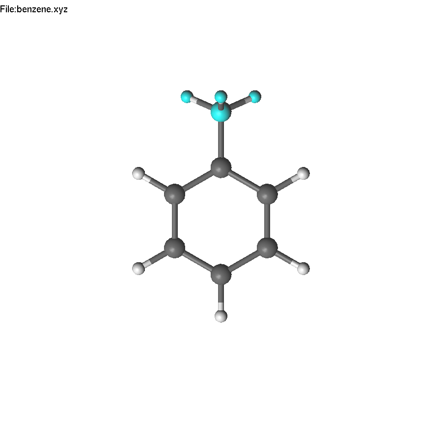
lgv contains a library of molecular fragments that can be added to a molecule. Press F3 to open the fragment picker. Fragments are organised into four visual categories, each with a coloured header bar: Fragments (building blocks with a Q anchor atom for attachment), Molecules (standalone structures inserted near the current molecule), Clusters, and Periodic (structures with lattice vectors). Click an icon to insert the corresponding fragment. For Fragments (with Q anchor): if one atom is selected the fragment is attached near that atom; if no atom is selected it is placed near the current molecule. For Molecules: if one atom is selected the molecule is placed near it; if atoms are present but none selected, click on the scene to choose the placement position; if the scene is empty the molecule is placed at the centre. Once a fragment has been selected, the Insert key re-inserts it without reopening the picker.

Operations with molecules and fragments

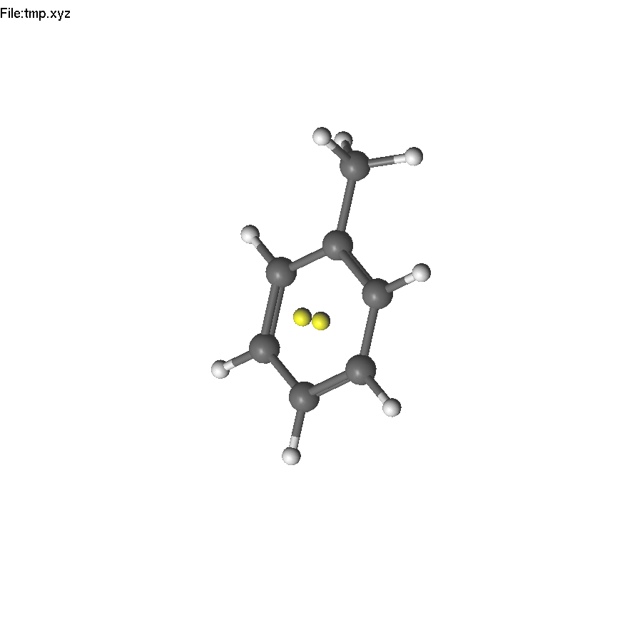
The task: create mesitylene (1,3,5-trimethylbenzene).

• run 'lgv -n benzene.xyz' or 'lgv -n'
• press F3 to invoke the menu with predefined molecules

  

• click on benzene (the rightmost icon in the first row)
• select one H atom

  

• press F3 again, and click on methyl group (CH3)

  

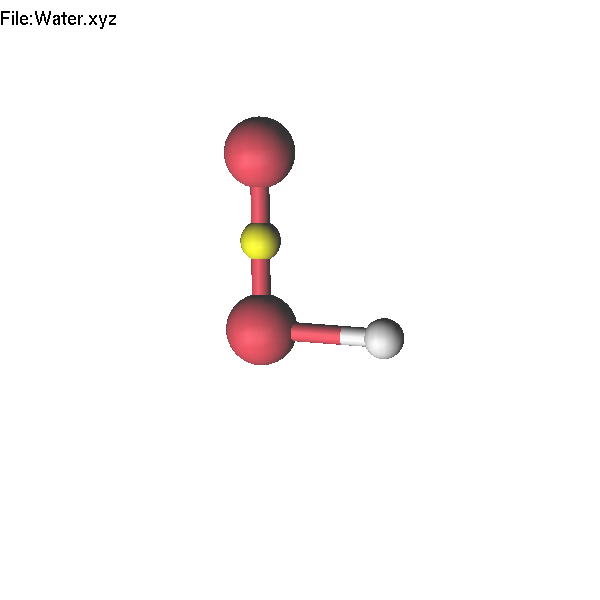
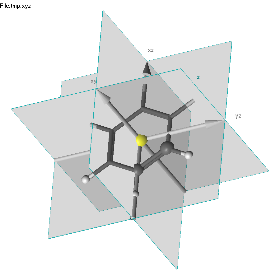
  Now we have to repeat the action, or use symmetry! The first step - we need to select a symmetry element, which we can use. It is the principal C6 axis. Unfortunately, there are no atoms on this axis, but we can create some. Select two opposite carbon atoms, and press End. This creates a dummy (yellow) atom in the center of the ring. Unselect (press Space).

  

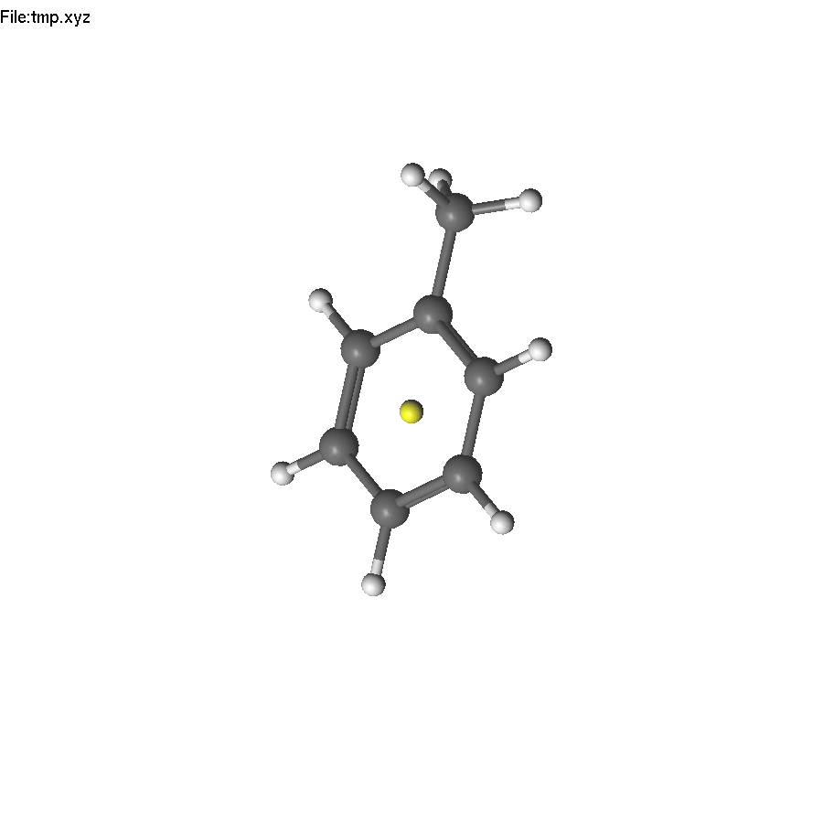
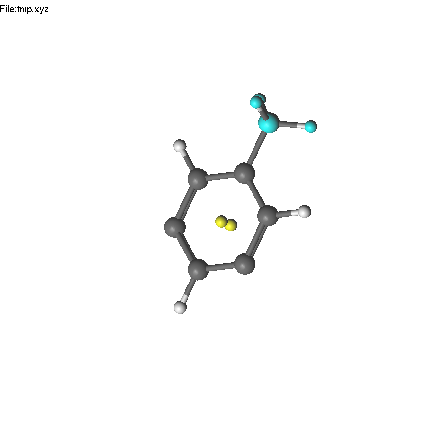
  Select the dummy atom and press PageUp, so it will jump from the plane. Repeat the operations to place another dummy atom back to the center.

  

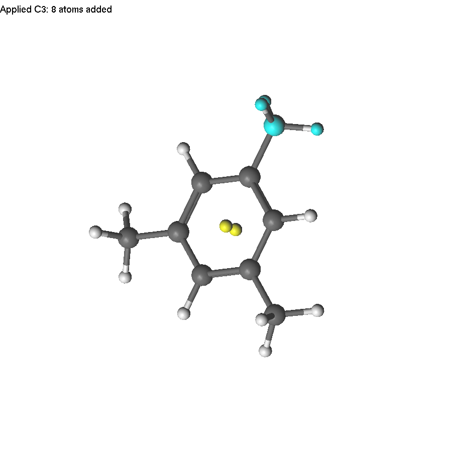
  Now select the two yellow atoms and press F8. A help line will appear (since there are several symmetry operations to be applied). Press 3 to use C3. The only problem is that applying the C3 operation also duplicates H atoms, which will become too close to carbon atoms. Therefore, we need to delete them first.

  

  Then select the axis, press F8, and press 3.

  

To modify coordinates via distances and angles, you may need dummy (reference) atoms. These dummy atoms can be added with the End key. If no atoms are selected, the 'End' key adds dummy atoms located on the X, Y, and Z axes. If a bond is selected, the dummy atom is placed in the middle of the bond. For example, if you have a planar molecule, but it is not oriented according to Cartesian axes, you can add dummy atoms on each axis, highlight all atoms in the molecule, and select a dihedral angle between the plane of the molecule and the desired plane created by the dummy atoms.

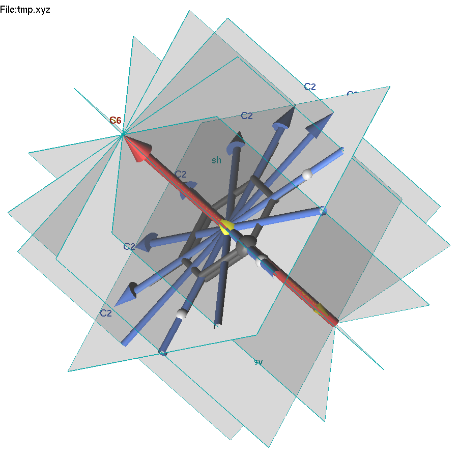
The lgv program can recognize the symmetry elements of a molecule, or apply symmetry operations for all, or highlighted atoms in the molecule. If no selection is made, F8 key displays symmetry elements of the molecule. Two symmetry engines are available: msym (default) and findsym. Press Shift-F8 to toggle between them. The fundamental difference between these two codes is that msym detects all symmetry operations, whereas findsym detects only abelian operations.

Also note that if a part of the molecule is highlighted, the symmetry operation will be applied only to the highlighted part.
In the example below, we highlighted two atoms and selected two others. F8 translates the highlighted group by the vector defined by the selected atoms.

Customization of lgv

lgv can be customized. Press the F9 key to save the current settings. It will create a directory .lgv-config in the current working directory with settings for colors, initial sizes, etc. These files can be edited to change the defaults. To share settings across all working directories, copy .lgv-config/ to $HOME/.lgv-config/. lgv will use the local directory when present, and fall back to the global one otherwise.

lgv can remember a ViewPoint (the current orientation of the molecule) and save it to a file. Later this file can be used to rotate another molecule accordingly. Use keys (v/V) to save or restore Viewpoint.

In some occasions, user would like to change the order of atoms in XYZ file. Although the simplest way to do this includes usage of editor, lgv provides some tools for resorting. If two atoms are selected, and # button pressed, selected atoms will exchange their order. Pressing # reorders atoms.

lgv provides several ways to modify the appearance of atoms. Highlight some atoms (Shift-click or rubber-band), then use the - / + keys to change their colour saturation:

• - once — pale (desaturated, washed-out)
• - twice / three times — more pale / very pale
• + once / twice / three times — vivid / more vivid / most vivid (increased saturation)

These modifiers are saved with the XYZ file as a suffix on the element name: C-, C--, C--- for pale levels; C+, C++, C+++ for vivid levels. The modifier is preserved across save/load cycles. The A key switches the overall atom rendering style.

Saving coordinates — the Save right-click menu offers three XYZ save variants in addition to the standard F2 / Shift-F2 keys:

• [F12] Save Oriented XYZ — applies the current screen rotation to all atom coordinates before saving, so the molecule's orientation as seen on screen is reflected in the file. The centroid is preserved.
• Save Canonical XYZ — writes a minimal, clean XYZ file: no #select / #axis / #Vec metadata lines, no dummy atoms (Z / Q / q / BQ), no pale/vivid modifiers. Useful when passing coordinates to other programs.

Double and triple bond display

lgv automatically detects double and triple bonds from molecular geometry using a valency-based algorithm (ported from LUSCUS):

1. Single bonds are detected by the standard distance threshold (1.15 × sum of covalent radii).
2. A second pass promotes SINGLE → DOUBLE for any bond where both endpoint atoms still have unsatisfied valency (counting bond orders: single=1, double=2, triple=3).
3. A third pass promotes DOUBLE → TRIPLE by the same criterion.

Bond-order multiplicity explicitly defined in fragment definitions (e.g. C=C in ethylene) takes priority over the auto-detection.

Pressing O (or using the right-click Options menu item Bond order: Auto / Single only) toggles between auto-detection and single-bonds-only mode. The setting is saved with F9.

Double-bond orientation: 3D vs Billboard

Double and triple bonds are drawn as two (or three) parallel cylinders. The offset direction can be set in two ways:

• 3D mode (default) — the offset lies in the plane defined by the bond and the nearest bonded neighbour atom. The parallel cylinders reflect true 3D geometry and rotate with the molecule.
• Billboard mode — the offset is always perpendicular to the bond and to the screen normal, so the two lines always appear side-by-side regardless of the viewing angle. Useful when bond-order legibility matters more than 3D accuracy.

Toggle via the right-click Options menu item Bond style: 3D / Billboard. The setting is saved with F9.

Electrostatic orientation of a highlighted group

After highlighting a group of atoms (e.g. a freshly inserted fragment), pressing E rotates the group around its centroid to minimise the pairwise Coulomb interaction with the rest of the molecule. The centroid position is not changed — only the orientation is optimised.

The algorithm uses a two-pass grid search over SO(3) (ZYZ Euler angles): a coarse pass at 24° steps, followed by a fine pass at 6° steps within ±36° of the coarse minimum. Charges used:

The feature works for any highlighted group, not only freshly inserted fragments. Press E again to re-run the search from the new orientation.

lgv understands several extensions of the XYZ format. Atom colour modifiers are written as a suffix on the element symbol (see above). At the end of an XYZ file the following #-prefixed lines may appear:

• #select i j … — atom indices to highlight on load
• #sphe x1 y1 z1 x2 y2 z2 — draw a sphere
• #axis x1 y1 z1 x2 y2 z2 — draw an axis
• #tria x1…z3 — draw a triangle
• #Orig / #Vec1 / #Vec2 / #Vec3 — lattice origin and vectors for periodic structures

The second line of an XYZ file (the comment line) is displayed as a second status bar line whenever it is non-empty and does not start with produced by. This is useful for files that store a title, formula, or energy in the comment field.

Tutorial: Loading CIF and SEWARD/GATEWAY files

lgv automatically recognises CIF and MOLCAS SEWARD/GATEWAY input files and converts them to XYZ internally — no external tools required.

CIF files (Crystallographic Information Files, extension .cif):

• Run lgv structure.cif
• lgv reads the unit cell, symmetry operators, and atomic coordinates, expands them into the asymmetric unit, and displays the result.

SEWARD/GATEWAY input files (MOLCAS input, typically .inp or any file containing &GATEWAY or &SEWARD):

• Run lgv molcas_input.inp
• lgv detects the &GATEWAY / &SEWARD marker, converts Basis Set and Xfield sections to XYZ (applying symmetry generators if present), and opens the result.

Tutorial: Periodic structures and cluster generation

When a coordinate file contains unit cell vectors (e.g. an XYZ file exported from a periodic calculation, or loaded from a CIF), lgv shows the cell axes on screen and enables cluster generation.

Bond drawing in periodic mode. In mixed-element structures (e.g. CsCl, NaCl) bonds between atoms of the same element are suppressed because they are usually non-physical. In single-element (elemental) structures such as copper or iron, this restriction is lifted and same-element bonds are drawn normally, so that the metal coordination environment is visible.

To generate a cluster of concentric shells around a chosen atom:

• Click on the atom that should be at the centre of the cluster (it will be highlighted in blue).
• Press C.
• lgv builds a supercell, cuts it into clusters of increasing radius (each adding one coordination shell), writes them to basename_clusters.molden, and immediately opens that file. The largest cluster is shown first. Cell axes are removed and the atom selection is cleared.

Use PageDown to step through smaller clusters (or PageUp for larger ones). The cluster frames are stored in Molden geo format, so all the Molden navigation keys apply.

Tutorial: MOPAC geometry optimization

lgv can drive a MOPAC semi-empirical geometry optimization and reload the result directly, without leaving the viewer. This requires the $MOPAC environment variable to point to the MOPAC binary.

Setup (once, e.g. in ~/.bashrc):

export MOPAC=/opt/mopac/mopac
export MOPAC_KEYWORDS="PM7 GNORM=0.01"   # optional; default is PM6

• Open an XYZ file in lgv.
• Make sure no atoms are selected (press Space or middle-click to deselect).
• Press M.
• lgv writes a .dat input file, runs MOPAC, parses the optimized Cartesian coordinates from the .out file, overwrites the .xyz file, and reloads it.

Note: this feature is not available in the WebAssembly build.

Tutorial: Watch mode (auto-reload)

Watch mode lets you monitor an ongoing calculation in real time. lgv polls the current file and automatically reloads it whenever the file changes on disk.

• Open the output XYZ file that your calculation is writing to (e.g. opt.xyz).
• Press F6 to start watching.
• Each time the calculation writes a new geometry, lgv reloads and displays it. Use m to animate through the accumulated frames.
• Press Shift-F6 to stop watching.

Watch mode works for XYZ, molden, and multi-frame files. It is particularly useful combined with m (animation) to see the trajectory build up as the calculation runs.

Record and Playback

lgv can record a session to a text file and play it back later. This is useful for creating reproducible demonstrations, automated tests, or batch processing scripts.

To start recording, launch lgv with:

lgv --record session.gvr molecule.xyz

All keyboard, mouse, and menu events are written to session.gvr with millisecond timestamps. To play back:

lgv --play session.gvr molecule.xyz

The playback file may also contain script directives (without timestamps) to control the session:

Lines beginning with # are treated as comments.

Batch Export and Headless Rendering (OSMesa build)

For server-side or automated rendering without a display, lgv can be compiled against the OSMesa off-screen rendering library:

make osmesa   (requires libosmesa6-dev)

The OSMesa build renders entirely in memory; no X11 display, GPU, or xvfb is needed. Combined with the -q flag, it exports PNG images and exits:

lgv -q -o all -v molecule.lus

This exports every orbital to separate PNG files named molecule_MO001.png, molecule_MO002.png, etc. The -v flag applies an automatic best viewpoint. The -o flag accepts all, a single number, or a comma-separated list of orbital numbers.

WebAssembly / Browser Build (Emscripten)

lgv can be compiled to WebAssembly for in-browser visualization:

make -f Makefile.emscripten   (requires Emscripten SDK)

The browser build provides the same core visualization features as the native build. Grid density differences (Diff menu in the toolbar) are fully supported: load a second .lus file, choose Minus or Plus and Same-space or Align (Kabsch rigid-body alignment), then click Compute Diff to display the result immediately.

Editing operations are accessible via the toolbar:

• The Actions XYZ dropdown provides: Help (F1), Clear selection (Space), Cancel/reset (Esc), Undo (Backspace), Fragment picker (F3), Insert atom/fragment (Ins), Delete selected atom (Del), Watch selected atoms (F6), Apply symmetry (F8).
• The Options dropdown includes Bond order: Auto/Single only and Bond style: 3D/Billboard in addition to the usual show/hide toggles.

The following features are not available in the WebAssembly version:

• MOPAC geometry optimization (key M) — requires a local binary.
• Sub-window multiview panels — the browser uses canvas overlays instead.
• Font mode cycling (key F) — font is fixed.
• Key remapping via lgv.keys file.
• Record/playback (--record / --play) — file access is sandboxed.

The JavaScript interface exposes functions such as gv_load_file, gv_compute_diff, gv_key_page_up, gv_save_png, gv_make_clusters, and others, allowing the browser UI to control lgv programmatically. PNG images are downloaded directly via the browser's download mechanism.

Visualization of orbitals with lgv

To visualize orbitals and densities with lgv, you have to compute a grid file (.grid) first using the GRID_IT program from the MOLCAS package.
Note that the quality of the picture depends on the keywords used in GRID_IT input.

Orbitals can be browsed with the PageUp/PageDown keys, or selected by a menu, invoked by the right mouse button. If you know the symmetry and number of the orbital you want to display, you can press the F4 (or =) key and then type # followed by the symmetry and orbital number, e.g. (# 1 3).

To change the isosurface value, you can use + or - key, or press F4 key, and type the desired isosurface value.

Sometimes you may want to filter the orbitals shown by lgv. Pressing Delete key you can hide an orbital. All hidden orbitals become visible again when the Insert key is pressed. Alternatively, you can apply a filter to hide some orbitals by a criterion: symmetry number (s), orbital energy (e), occupation number (o), or typeindex (i). The use of filters is clear from the following examples: Press the F4 key and type #: followed by a filter command - #:s14 to display orbitals only from symmetry 1 and 4, #:e-2:1 to display orbitals in an energy range between -2 and 1.

When the grid file is loaded, lgv displays subspaces (frozen, inactive, RAS1, RAS2, RAS3, secondary, deleted). The user can modify the type index of the orbital, save (F2 key) the INPORB file (it will have an extension GvOrb), and use this file in a subsequent RASSCF calculation without having to reorder the orbitals. In order to modify the index of the displayed orbital, user can use a menu, or press one of the keys: fi123sd. Pressing Space key (or middle mouse button) changes the type index in a loop.

It is possible to display all orbitals of the grid file simultaneously. Press the F3 key to get the screen with all orbitals.

By default, the background (rainbow colors) for each orbital corresponds to the type index information. Clicking on an individual orbital you can use the same keys to modify it's type, or delete it from the screen. Pressing F3 button again, or Escape will close the multiview mode. Using PageUp/PageDown in multiview mode will increase/decrease the sizes of subscreens. These features of lgv can be quite helpful for selecting the different orbital spaces in RASSCF calculations.

lgv can also be used to compare densities from different GRID_IT calculations. A command lgv --minus scf.grid rasscf.grid --out diff.grid computes the density difference (SCF − RASSCF) and writes it to diff.grid. The shorthand flags --minus and --plus are equivalent to -a -1 and -a 1 respectively.

The simplest case requires both grid files to have the same mesh (same Net= dimensions). If the two calculations used the same coordinate frame but different mesh resolutions, add --same-space: lgv will trilinearly resample the first grid onto the second grid’s mesh before forming the linear combination.

If the two densities come from slightly different molecular geometries (e.g. consecutive steps of a geometry optimisation or points along an IRC path), use --align. lgv checks that both files contain the same atoms in the same order, verifies that no atom has moved more than the displacement tolerance (default 2 Å, overridden with --align-tol), and then computes an optimal rigid-body transformation (Kabsch rotation + translation) from the paired atom positions. Grid2 is resampled onto grid1’s coordinate frame using trilinear interpolation, the linear combination is formed, and the result is written on grid1’s mesh with grid1’s atom positions. The alignment RMSD is printed to stderr so you can check whether the fit is reasonable:

lgv --align --minus step_001.grid step_002.grid --out ddiff.grid

For the interaction-density workflow (comparing the density of a complex AB to the sum of its fragments A and B in ghost-atom calculations) the grids must share the same coordinate frame. Compute the fragment sum first: lgv --plus A.grid B.grid --out sum.grid, then subtract it from the complex: lgv --minus AB.grid sum.grid --out interaction.grid.

Electrostatic Potential (ESP) Surface

lgv can compute and display an electrostatic potential (ESP) surface: a Gaussian-blended van der Waals isosurface colored by the Coulomb potential, with red for electron-rich (negative) regions and blue for electron-poor (positive) regions. The ESP is computed as

E(r) = ∑_i q_i / |r − r_i|

where q_i are point charges at the atomic positions. Three sources of charges are supported.

From Molden charges (Mulliken or LoProp)

If a .molden file is loaded that contains a [CHARGE] (MULLIKEN) or [CHARGE] (LOPROP) section, the ESP surface can be computed directly:

• Right-click → ESP surface → Compute from Molden charges (native build).
• In the browser build, use the Actions menu → ESP surface (Molden charges).

LoProp charges (if present) are preferred over Mulliken charges when both sections exist.

From an XYZ+charges file

A plain-text file with one atom per line in the format

N
comment
Element  x  y  z  charge
...

where coordinates are in Ångström and charges in electron units (e), can be loaded via Right-click → ESP surface → From XYZ+charges file (native) or the Actions menu in the browser build (upload button).

From a Gaussian Cube EPOT file

A Gaussian Cube file (.cube) containing an electrostatic potential grid — as produced by Gaussian, ORCA, or similar programs — can be loaded via Right-click → ESP surface → From EPOT grid (Cube format) or the Actions menu in the browser build (upload button). The atom positions from the currently loaded file are used for the van der Waals surface; the cube grid values are interpolated onto the surface vertices by trilinear interpolation. Cube coordinates are converted from Bohr to Ångström and values from e/Bohr to e/Å automatically. The color range is auto-scaled from the cube data.

Generating an ESP grid from a Molden file (Python script)

The script molden2esp_lus.py (included in the lgv distribution) reads atom positions and Mulliken/LoProp charges from a Molden file, computes the Coulomb ESP on a 3-D grid, and writes a Luscus .lus file with GridName= Electrostatic that can be loaded into lgv as a regular grid file for isosurface display:

python3 molden2esp_lus.py scf.molden esp.lus
python3 molden2esp_lus.py scf.molden esp.lus --step 0.2 --pad 3.0

The --step option sets the grid spacing in Ångström (default 0.25) and --pad sets the margin beyond the van der Waals radius of each atom (default 3.0 Å). The script requires only the Python standard library.

Controlling the ESP display

The color mapping uses three parameters (defined in esp.c):

• esp_max_value — ESP magnitude (e/Å) at which the color reaches full saturation (default 0.10).
• esp_white_region — ESP magnitude below which the surface appears white (default 0.025).
• esp_color_pos — RGBA color for positive ESP (default blue, 0,0,1,0.7).
• esp_color_neg — RGBA color for negative ESP (default red, 1,0,0,0.7).

Use Show/Hide ESP surface to toggle visibility without discarding the computed surface, and Clear ESP surface to remove it. Loading a new file clears the ESP surface automatically.