


MOLCAS manual: Next: 10.5 Excited states. Up: 10. Examples Previous: 10.3 Computing a reaction path.
Here we will give an example of how geometrical structures obtained at
one level of theory can be used in an analysis at high quality wave functions.
Table | |||||||||||||||||||||||||||||||||||||||||||||||||||||||||||||||||||||||||||||||||||||||||||||||||||||||||||||||||||||||||||||||||||||||||||||||||||||||||||||||||||||||||||||||||||||||||||||||||||||||||||||||||||||||||||||||||||||||||||||||||||||||||||||||||||||||||||||||||||||||||||||||||||||||||||||||||||||||||||||||||||||||||||||||||||||||||||||||||||||||||||||||||||||||||||||||||||||||||||||||||||||||||||||||||||||||||||||||||||||||||||||||||||||||||||||||||||||
| C1C3 | C1C2 | C2C1C3 | C1C3H6 | C2C1C3H6 | C2H5 | C1H5 | C1C2H5 | C3C1C2H5 | |
| Dimethylcarbene | |||||||||
| CASb | 1.497 | 1.497 | 110.9 | 102.9 | 88.9 | 1.099 | 102.9 | 88.9 | |
| MP2c | 1.480 | 1.480 | 110.3 | 98.0 | 85.5 | 1.106 | 98.0 | 85.5 | |
| Transition structure | |||||||||
| CASb | 1.512 | 1.394 | 114.6 | 106.1 | 68.6 | 1.287 | 1.315 | 58.6 | 76.6 |
| MP2c | 1.509 | 1.402 | 112.3 | 105.1 | 69.2 | 1.251 | 1.326 | 59.6 | 77.7 |
| Propene | |||||||||
| CASb | 1.505 | 1.344 | 124.9 | 110.7 | 59.4 | ||||
| MP2c | 1.501 | 1.338 | 124.4 | 111.1 | 59.4 | ||||
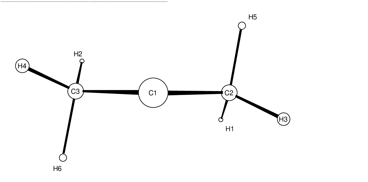
aC1, carbenoid center; C2, carbon which looses the hydrogen H5. See Figure ![[*]](crossref.png) . . |
|||||||||
| bPresent results. CASSCF, ANO-S C 3s2p1d, H 2d1p. Two electrons in two orbitals. | |||||||||
| cMP2 6-31G(2p,d), Ref. [255]. | |||||||||
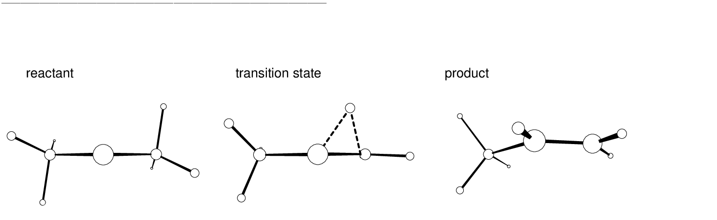
The main structural effects occurring during the reaction can be observed
displayed in Table . As the rearrangement starts out one
hydrogen atom (H5) moves in a plane almost perpendicular to the plane
formed by the three carbon atoms while the remaining two hydrogen atoms
on the same methyl group swing very rapidly into a nearly planar
position (see Figure on page ).
As the  bond is formed we observe
a contraction of the C1-C2 distance. In contrast, the spectator
methyl group behaves as a rigid body. Their parameters were
not compiled here but it rotates and bends slightly [255]. Focusing
on the second half reaction, the moving hydrogen atom rotates into the
plane of the carbon atoms to form the new C1-H5 bond. This movement
is followed by a further shortening of the preformed C1-C2 bond,
which acquires the bond distance of a typical double carbon bond, and
smaller adjustments in the positions of the other atoms. The structures
of the reactant, transition state, and product are shown in
Figure .
bond is formed we observe
a contraction of the C1-C2 distance. In contrast, the spectator
methyl group behaves as a rigid body. Their parameters were
not compiled here but it rotates and bends slightly [255]. Focusing
on the second half reaction, the moving hydrogen atom rotates into the
plane of the carbon atoms to form the new C1-H5 bond. This movement
is followed by a further shortening of the preformed C1-C2 bond,
which acquires the bond distance of a typical double carbon bond, and
smaller adjustments in the positions of the other atoms. The structures
of the reactant, transition state, and product are shown in
Figure .
As was already mentioned we will apply now higher-correlated methods for the reactant, product, and transition state system at the CASSCF optimized geometries to account for more accurate relative energies. In any case a small basis set has been used and therefore the goal is not to be extremely accurate. For more complete results see Ref. [255]. We are going to perform calculations with the MP2, MRCI, ACPF, CASPT2, CCSD, and CCSD(T) methods.
Starting with dimethylcarbene, we will use the following input file:
&SEWARD &END
Title
Dimethylcarbene singlet C2-sym
CASSCF(ANO-VDZP) opt geometry
Symmetry
XY
Basis set
C.ANO-S...3s2p1d.
C1 .0000000000 .0000000000 1.2019871414
C2 .0369055124 2.3301037548 -.4006974719
End of basis
Basis set
H.ANO-S...2s1p.
H1 -.8322309260 2.1305589948 -2.2666729831
H2 -.7079699536 3.9796589218 .5772009623
H3 2.0671154914 2.6585385786 -.6954193494
End of basis
PkThrs
1.0E-10
End of input
&SCF &END
Title
Dmc
Occupied
7 5
End of input
&RASSCF &END
Title
Dmc
Symmetry
1
Spin
1
Nactel
2 0 0
Inactive
6 5
Ras2
1 1
Thrs
1.0E-05,1.0E-03,1.0E-03
Iteration
50,25
LumOrb
End of input
&CASPT2 &END
Title
Dmc
LRoot
1
Frozen
2 1
End of input
&MOTRA &END
Title
Dmc
Frozen
2 1
JobIph
End of input
&GUGA &END
Title
Dmc
Electrons
18
Spin
1
Inactive
4 4
Active
1 1
Ciall
1
Print
5
End of input
&MRCI &END
Title
Dimethylcarbene
SDCI
End of input
&MRCI &END
Title
Dimethylcarbene
ACPF
End of input
* Now we generate the single ref. function
* for coupled-cluster calculations
&RASSCF &END
Title
Dmc
Symmetry
1
Spin
1
Nactel
0 0 0
Inactive
7 5
Ras2
0 0
Thrs
1.0E-05,1.0E-03,1.0E-03
Iteration
50,25
LumOrb
OutOrbitals
Canonical
End of input
&MOTRA &END
Title
Dmc
Frozen
2 1
JobIph
End of input
&CCSDT &END
Title
Dmc
CCT
Iterations
40
Triples
2
End of input
Observe in the previous input that we have generated a multiconfigurational
wave function for CASPT2, MRCI, and ACPF wave functions but a single configuration
reference wave function (using RASSCF program with the options
OUTOrbitals and CANOnical)
for the CCSD and CCSD(T) wave functions. Notice also
that to compute a multiconfigurational ACPF wave function we have to use
the MRCI program, not the CPF module which does not accept
more than one single reference. In all the highly correlated
methods we have frozen the three carbon core orbitals because of the reasons
already explained in section . For MRCI, ACPF, CCSD, and CCSD(T)
the freezing is performed in the MOTRA step.
One question that can be addressed is which is the proper reference space
for the multiconfigurational calculations. As was explained when we selected
the active space for the geometry optimizations, we performed several tests
at different stages in the reaction path and observed that the smallest
meaningful active space, two electrons in two orbitals, was sufficient
in all the cases. We can come back to this problem here to select the
reference for CASPT2, MRCI, and ACPF methods. The simple analysis of the
SCF orbital energies shows that in dimethylcarbene, for instance, the
orbital energies of the C-H bonds are close to those of the C-C  bonds and additionally those orbitals are strongly mixed along
the reaction path. A balanced active space including all orbitals necessary
to describe the shifting H-atom properly would require a full valence
space of 18 electrons in 18 orbitals. This is not a feasible space, therefore
we proceed with the minimal active space and analyze later the quality
of the results. The CASSCF wave function will then include for dimethylcarbene
and the transition state structure the ()2()0 and
()0()2 configurations correlating the non-bonded electrons
localized at the carbenoid center where as for propene the active space
include the equivalent valence space.
bonds and additionally those orbitals are strongly mixed along
the reaction path. A balanced active space including all orbitals necessary
to describe the shifting H-atom properly would require a full valence
space of 18 electrons in 18 orbitals. This is not a feasible space, therefore
we proceed with the minimal active space and analyze later the quality
of the results. The CASSCF wave function will then include for dimethylcarbene
and the transition state structure the ()2()0 and
()0()2 configurations correlating the non-bonded electrons
localized at the carbenoid center where as for propene the active space
include the equivalent valence space.
The GUGA input must be built carefully. There are several ways to specify the reference configurations for the following methods. First, the keyword ELECtrons refers to the total number of electrons that are going to be correlated, that is, all except those frozen in the previous MOTRA step. Keywords INACtive and ACTIve are optional and describe the number of inactive (occupation two in all the reference configurations) and active (varying occupation number in the reference configurations) orbitals of the space. Here ACTIve indicates one orbital of each of the symmetries. The following keyword CIALl indicates that the reference space will be the full CI within the subspace of active orbitals. It must be always followed by symmetry index (number of the irrep) for the resulting wave function, one here.
For the transition state structure we do not impose any symmetry restriction, therefore the calculations are performed in the C1 group with the input file:
&SEWARD &END
Title
Dimethylcarbene to propene
Transition State C1 symmetry
CASSCF (ANO-VDZP) opt geometry
Basis set
C.ANO-S...3s2p1d.
End of basis
Basis set
H.ANO-S...2s1p.
End of basis
PkThrs
1.0E-10
End of input
&SCF &END
Title
Ts
Occupied
12
End of input
&MBPT2 &END
Title
Ts
Frozen
3
End of input
&RASSCF &END
Title
Ts
Symmetry
1
Spin
1
Nactel
2 0 0
Inactive
11
Ras2
2
Iteration
50,25
LumOrb
End of input
&CASPT2 &END
Title
Ts
LRoot
1
Frozen
3
End of input
&MOTRA &END
Title
Ts
Frozen
3
JobIph
End of input
&GUGA &END
Title
Ts
Electrons
18
Spin
1
Inactive
8
Active
2
Ciall
1
Print
5
End of input
&MRCI &END
Title
Ts
SDCI
End of input
&MRCI &END
Title
Ts
ACPF
End of input
&RASSCF &END
Title
Ts
Symmetry
1
Spin
1
Nactel
0 0 0
Inactive
12
Ras2
0
Iteration
50,25
LumOrb
OutOrbitals
Canonical
End of input
&MOTRA &END
Title
Ts
Frozen
3
JobIph
End of input
&CCSDT &END
Title
Ts
CCT
Iterations
40
Triples
2
End of input
Finally we compute the wave functions for the product, propene, in the Cs symmetry group with the input:
&SEWARD &END
Title
Propene singlet Cs-sym
CASSCF(ANO-VDZP) opt geometry
Symmetry
Z
Basis set
C.ANO-S...3s2p1d.
C1 -2.4150580342 .2276105054 .0000000000
C2 .0418519070 .8733601069 .0000000000
C3 2.2070668305 -.9719171861 .0000000000
End of basis
Basis set
H.ANO-S...2s1p.
H1 -3.0022907382 -1.7332097498 .0000000000
H2 -3.8884900111 1.6454331428 .0000000000
H3 .5407865292 2.8637419734 .0000000000
H4 1.5296107561 -2.9154199848 .0000000000
H5 3.3992878183 -.6985812202 1.6621549148
End of basis
PkThrs
1.0E-10
End of input
&SCF &END
Title
Propene
Occupied
10 2
End of input
&MBPT2 &END
Title
Propene
Frozen
3 0
End of input
&RASSCF &END
Title
Propene
Symmetry
1
Spin
1
Nactel
2 0 0
Inactive
10 1
Ras2
0 2
Thrs
1.0E-05,1.0E-03,1.0E-03
Iteration
50,25
LumOrb
End of input
&CASPT2 &END
Title
Propene
LRoot
1
Frozen
3 0
End of input
&MOTRA &END
Title
Propene
Frozen
3 0
JobIph
End of input
&GUGA &END
Title
Propene
Electrons
18
Spin
1
Inactive
7 1
Active
0 2
Ciall
1
Print
5
End of input
&MRCI &END
Title
Propene
SDCI
End of input
&MRCI &END
Title
Propene
ACPF
End of input
&RASSCF &END
Title
Propene
Symmetry
1
Spin
1
Nactel
0 0 0
Inactive
10 2
Ras2
0 0
Thrs
1.0E-05,1.0E-03,1.0E-03
Iteration
50,25
LumOrb
OutOrbitals
Canonical
End of input
&MOTRA &END
Title
Propene
Frozen
3 0
JobIph
End of input
&CCSDT &END
Title
Propene
CCT
Iterations
40
Triples
2
End of input
Table compiles the total and relative energies
obtained for the studied reaction at the different levels of
theory employed.
| Single configurational methods | ||||
| method | RHF | MP2 | CCSD | CCSD(T) |
| Dimethylcarbene | ||||
| -117.001170 | -117.392130 | -117.442422 | -117.455788 | |
| Transition state structure | ||||
| -116.972670 | -117.381342 | -117.424088 | -117.439239 | |
| BHa | (17.88) | (6.77) | (11.50) | (10.38) |
| Propene | ||||
| -117.094700 | -117.504053 | -117.545133 | -117.559729 | |
| EXb | (-58.69) | (-70.23) | (-64.45) | (-65.22) |
| Multiconfigurational methods | ||||
| method | CASSCF | CASPT2 | SD-MRCI+Q | ACPF |
| Dimethylcarbene | ||||
| -117.020462 | -117.398025 | -117.447395 | -117.448813 | |
| Transition state structure | ||||
| -116.988419 | -117.383017 | -117.430951 | -117.432554 | |
| BHa | (20.11) | (9.42) | (10.32) | (10.20) |
| Propene | ||||
| -117.122264 | -117.506315 | -117.554048 | -117.554874 | |
| EXb | (-63.88) | (-67.95) | (-66.93) | (-66.55) |
| aBarrier height. Needs to be corrected with the zero point vibrational correction. | ||||
| bExothermicity. Needs to be corrected with the zero point vibrational correction. | ||||
We can discuss now the quality of the results obtained and their
reliability (for a more careful discussion of the accuracy of
quantum chemical calculations see Ref. [244]).
In first place we have to consider that a valence
double-zeta plus polarization basis set is somewhat small to obtain
accurate results. At least a triple-zeta quality would be required.
The present results have, however, the goal to serve as an example.
We already pointed out that the CASSCF geometries were very similar
to the MP2 reported geometries [255]. This fact validates
both methods. MP2 provides remarkably accurate geometries using
basis sets of triple-zeta quality, as in Ref. [255], in
situations were the systems can be described as singly configurational,
as the CASSCF calculations show. The Hartree-Fock configuration has
a contribution of more than 95% in all three structures, while the
largest weight for another configuration appears in propene for
()0( )2 (4.2%).
The MRCI calculations provide also one test of the validity of the reference wave function. For instance, the MRCI output for propene is:
FINAL RESULTS FOR STATE NR 1
CORRESPONDING ROOT OF REFERENCE CI IS NR: 1
REFERENCE CI ENERGY: -117.12226386
EXTRA-REFERENCE WEIGHT: .11847074
CI CORRELATION ENERGY: -.38063043
CI ENERGY: -117.50289429
DAVIDSON CORRECTION: -.05115380
CORRECTED ENERGY: -117.55404809
ACPF CORRECTION: -.04480105
CORRECTED ENERGY: -117.54769535
CI-COEFFICIENTS LARGER THAN .050
NOTE: THE FOLLOWING ORBITALS WERE FROZEN
ALREADY AT THE INTEGRAL TRANSFORMATION STEP
AND DO NOT EXPLICITLY APPEAR:
SYMMETRY: 1 2
PRE-FROZEN: 3 0
ORDER OF SPIN-COUPLING: (PRE-FROZEN, NOT SHOWN)
(FROZEN, NOT SHOWN)
VIRTUAL
ADDED VALENCE
INACTIVE
ACTIVE
ORBITALS ARE NUMBERED WITHIN EACH SEPARATE SYMMETRY.
CONFIGURATION 32 COEFFICIENT -.165909 REFERENCE
SYMMETRY 1 1 1 1 1 1 1 2 2 2
ORBITALS 4 5 6 7 8 9 10 1 2 3
OCCUPATION 2 2 2 2 2 2 2 2 0 2
SPIN-COUPLING 3 3 3 3 3 3 3 3 0 3
CONFIGURATION 33 COEFFICIENT -.000370 REFERENCE
SYMMETRY 1 1 1 1 1 1 1 2 2 2
ORBITALS 4 5 6 7 8 9 10 1 2 3
OCCUPATION 2 2 2 2 2 2 2 2 1 1
SPIN-COUPLING 3 3 3 3 3 3 3 3 1 2
CONFIGURATION 34 COEFFICIENT .924123 REFERENCE
SYMMETRY 1 1 1 1 1 1 1 2 2 2
ORBITALS 4 5 6 7 8 9 10 1 2 3
OCCUPATION 2 2 2 2 2 2 2 2 2 0
SPIN-COUPLING 3 3 3 3 3 3 3 3 3 0
**************************************************************
The Hartree-Fock configuration contributes to the MRCI configuration with a weight of 85.4%, while the next configuration contributes by 2.8%. Similar conclusions can be obtained analyzing the ACPF results and for the other structures. We will keep the MRCI results including the Davidson correction (MRCI+Q) which corrects for the size-inconsistency of the truncated CI expansion [244].
For CASPT2 the evaluation criteria were already commented in
section . The portion of the CASPT2 output for
propene is:
Reference energy: -117.1222638304
E2 (Non-variational): -.3851719971
E2 (Variational): -.3840516039
Total energy: -117.5063154343
Residual norm: .0000000000
Reference weight: .87905
Contributions to the CASPT2 correlation energy
Active & Virtual Only: -.0057016698
One Inactive Excited: -.0828133881
Two Inactive Excited: -.2966569393
----------------------------------------------------------------------------
Report on small energy denominators, large components, and large energy contributions.
The ACTIVE-MIX index denotes linear combinations which gives ON expansion functions
and makes H0 diagonal within type.
DENOMINATOR: The (H0_ii - E0) value from the above-mentioned diagonal approximation.
RHS value: Right-Hand Side of CASPT2 Eqs.
COEFFICIENT: Multiplies each of the above ON terms in the first-order wave function.
Thresholds used:
Denominators: .3000
Components: .0250
Energy contributions: .0050
CASE SYMM ACTIVE NON-ACT IND DENOMINATOR RHS VALUE COEFFICIENT CONTRIBUTION
AIVX 1 Mu1.0003 In1.004 Se1.022 2.28926570 .05988708 -.02615995 -.00156664
The weight of the CASSCF reference to the first-order wave function is
here 87.9%, very close to the weights obtained for the dimethylcarbene and
the transition state structure,
and there is only a small contribution to the wave function and energy
which is larger than the selected thresholds. This should not be considered as a
intruder state, but as a contribution from the fourth inactive orbital which
could be, eventually, included in the active space. The contribution to the
second-order energy in this case is smaller than 1 Kcal/mol. It can be observed
that the same contribution shows up for the transition state structure but not
for the dimethylcarbene. In principle this could be an indication that a larger
active space, that is, four electrons in four orbitals, would give a slightly
more accurate CASPT2 energy. The present results will probably overestimate
the second-order energies for the transition state structure and the propene,
leading to a slightly smaller activation barrier and a slightly larger
exothermicity, as can be observed in Table . The orbitals
pointed out as responsible for the large contributions in propene are the
fourth inactive and 22nd secondary orbitals of the first symmetry. They are
too deep and too high, respectively, to expect that an increase in the active
space could in fact represent a great improvement in the CASPT2 result.
In any case we tested for four orbitals-four electrons CASSCF/CASPT2 calculations
and the results were very similar to those presented here.
Finally we can analyze the so-called  -diagnostic [256]
for the coupled-cluster wave functions. is defined for closed-shell
coupled-cluster methods as the Euclidean norm of the vector of T1
amplitudes normalized by the number of electrons correlated:
-diagnostic [256]
for the coupled-cluster wave functions. is defined for closed-shell
coupled-cluster methods as the Euclidean norm of the vector of T1
amplitudes normalized by the number of electrons correlated:
 .
In the output of the CCSD program we have:
.
In the output of the CCSD program we have:
Convergence after 17 Iterations
Total energy (diff) : -117.54513288 -.00000061
Correlation energy : -.45043295
E1aa contribution : .00000000
E1bb contribution : .00000000
E2aaaa contribution : -.04300448
E2bbbb contribution : -.04300448
E2abab contribution : -.36442400
Five largest amplitudes of :T1aa
SYMA SYMB SYMI SYMJ A B I J VALUE
2 0 2 0 4 0 2 0 -.0149364994
2 0 2 0 2 0 2 0 .0132231037
2 0 2 0 8 0 2 0 -.0104167047
2 0 2 0 7 0 2 0 -.0103366543
2 0 2 0 1 0 2 0 .0077537734
Euclidean norm is : .0403635306
Five largest amplitudes of :T1bb
SYMA SYMB SYMI SYMJ A B I J VALUE
2 0 2 0 4 0 2 0 -.0149364994
2 0 2 0 2 0 2 0 .0132231037
2 0 2 0 8 0 2 0 -.0104167047
2 0 2 0 7 0 2 0 -.0103366543
2 0 2 0 1 0 2 0 .0077537734
Euclidean norm is : .0403635306
In this case T1aa and T1bb are identical because we are computing a
closed-shell singlet state. The five largest T1 amplitudes are
printed, as well as the Euclidean norm. Here the number of correlated
electrons is 18, therefore the value for the diagnostic is 0.01.
This value can be considered acceptable as evaluation of the
quality of the calculation. The use of as a diagnostic is
based on an observed empirical correlation: larger values give poor
CCSD results for molecular structures, binding energies, and
vibrational frequencies [257]. It was considered that values
larger than 0.02 indicated that results from single-reference electron
correlation methods limited to single and double excitations should be
viewed with caution.
There are several considerations concerning the diagnostic
[256]. First, it is only valid within the frozen core
approximation and it was defined for coupled-cluster procedures
using SCF molecular orbitals in the reference function. Second, it is
a measure of the importance of non-dynamical electron correlation effects
and not of the degree of the multireference effects. Sometimes the two
effects are related, but not always (see discussion in Ref. [257]).
Finally, the performance of the CCSD(T) method is reasonably good even
in situations where has a value as large as 0.08.
In conclusion, the use of together with other wave function
analysis, such as explicitly examining the largest T1 and T2
amplitudes, is the best approach to evaluate the quality of the
calculations but this must be done with extreme caution.
As the present systems are reasonably well described by a single
determinant reference function there is no doubt that the CCSD(T)
method provides the most accurate results. Here CASPT2, MRCI+Q,
ACPF, and CCSD(T) predict the barrier height from the reactant
to the transition state with an accuracy better than 1 Kcal/mol.
The correspondence is somewhat worse, about 3 Kcal/mol, for the
exothermicity. As the difference is largest for the CCSD(T) method
we may conclude than triple and higher order excitations are of
importance to achieve a balanced correlation treatment, in particular
with respect to the partially occupied orbital at the
carbenoid center. It is also noticeable that the relative MP2
energies appear to be shifted about 3-4 Kcal/mol towards lower
values. This effect may be due to the overestimation of the
hyper-conjugation effect which appears to be strongest in dimethylcarbene
[258,255].
Additional factors affecting the accuracy of the results obtained are the zero point vibrational energy correction and, of course, the saturation of the one particle basis sets. The zero point vibrational correction could be computed by performing a numerical harmonic vibrational analysis at the CASSCF level using MOLCAS. At the MP2 level [255] the obtained values were -1.1 Kcal/mol and 2.4 Kcal/mol for the activation barrier height and exothermicity, respectively. Therefore, if we take as our best values the CCSD(T) results of 10.4 and -65.2 Kcal/mol, respectively, our prediction would be an activation barrier height of 9.3 Kcal/mol and an exothermicity of -62.8 Kcal/mol. Calculations with larger basis sets and MP2 geometries gave 7.4 and -66.2 Kcal/mol, respectively [255]. The experimental estimation gives a lower limit to the activation barrier of 3.3 Kcal/mol [255].
MOLCAS provides also a number of one-electron properties
which can be useful to analyze the chemical behavior of the systems.
For instance, the Mulliken population analysis is available for the
RHF, CASSCF, CASPT2, MRCI, and ACPF wave functions. Mulliken charges
are known to be strongly biased by the choice of the basis sets,
nevertheless one can restrict the analysis to the relative charge
differences during the course of the reaction to obtain a qualitative
picture. We can use, for instance, the charge distribution obtained
for the MRCI wave function, which is listed in Table .
Take into account that the absolute values of the charges can
vary with the change of basis set.
| C2a | C1b | H5c |  |
H1+H3e | Mef | ||
| Dimethylcarbene | |||||||
| -0.12 | -0.13 | 0.05 | -0.20 | 0.14 | 0.07 | ||
| Transition state structure | |||||||
| -0.02 | -0.23 | 0.05 | -0.20 | 0.17 | 0.02 | ||
| Propene | |||||||
| -0.18 | -0.02 | 0.05 | -0.15 | 0.18 | -0.02 | ||
| aCarbon from which the hydrogen is withdrawn. | |||||||
| bCentral carbenoid carbon. | |||||||
| cMigrating hydrogen. | |||||||
| dSum of charges for centers C2, C1, and H5. | |||||||
| eSum of charges for the remaining hydrogens attached to C2. | |||||||
| fSum of charges for the spectator methyl group. | |||||||
In dimethylcarbene both the medium and terminal carbons appear equally charged.
During the migration of hydrogen H5 charge flows from the hydrogen donating
carbon, C2, to the carbenoid center. For the second half of the reaction
the charge flows back to the terminal carbon from the centered carbon, probably
due to the effect of the delocalization.
Next: 10.5 Excited states. Up: 10. Examples Previous: 10.3 Computing a reaction path.