8.41 rasscf

The RASSCF program in MOLCAS performs multiconfigurational SCF calculations using the Restricted Active Space [83] or the Generalized Active Space [13] SCF construction of the wave function. RASSCF is an extension of the Complete Active Space (CAS) approach, in which the wave function is obtained as a full CI expansion in an active orbital space [84,85]. The RASSCF method is based on a partitioning of the occupied molecular orbitals into the following groups:

CASSCF calculations can be performed with the program, by allowing orbitals only in the RAS2 space. A single reference SDCI wave function is obtained by allowing a maximum of 2 holes in RAS1 and a maximum of 2 electrons in RAS3, while RAS2 is empty (the extension to SDT- and SDTQ-CI is obvious). Multireference CI wave functions can be constructed by adding orbitals also in RAS2.

The RASSCF program is based on the split GUGA formalism. However, it uses determinant based algorithms to solve the configuration interaction problem [71]. To ensure a proper spin function, the transformation to a determinant basis is only performed in the innermost loops of the program to evaluate the $\sigma$ -vectors in the Davidson procedure and to compute the two-body density matrices. The upper limit to the size of the CASSCF wave function that can be handled with the present program is about 10⁷ CSFs and is, in general, limited by the dynamic work array available to the program.

The orbital optimization in the RASSCF program is performed using the super-CI method. The reader is referred to the references [83,86] for more details. A quasi-Newton (QN) update method is used in order to improve convergence. No explicit CI-orbital coupling is used in the present version of the program, except for the coupling introduced in the QN update.

Convergence of the orbital optimization procedure is normally good for CASSCF type wave functions, but problems can occur in calculations on excited states, especially when several states are close in energy. In such applications it is better to optimize the orbitals for the average energy of several electronic states. Further, convergence can be slower in some cases when orbitals in RAS1 and RAS3 are included. The program is not optimal for SDCI calculations with a large number of orbitals in RAS1 and RAS3.

As with other program modules, please observe that the input is preprocessed and may therefore differ in some respects to the input file prepared by the user. In most cases, this does not imply any functional changes as compared to the user's requests. However, when the input has some minor mistakes or contradictory requests, it can be modified when it is felt that the correction is beneficial. Also, see below for the keyword EXPERT. Without this keyword, the program is assuming more flexibility to optimize the calculation, e.g. by using CIRESTART, if the RASSCF module is called during a numerical differentiation, even if the input requested doing CI calculations from scratch. Using keyword EXPERT, such automatic modification of the user's input is no longer done, and the input is obeyed exactly (when possible).

It is best to provide a set of good input orbitals. (The program can be started from scratch by using CORE, but this should be used only if other possibilities fail). They can either be from some other type of calculation, for example SCF, or generated by GUESSORB, or from a previous RASSCF calculation on the same system. In the first case the orbitals are normally given in formatted form, file INPORB, in the second case they can also be read from a RASSCF input unit JOBOLD. Input provides both possibilities. Some care has to be taken in choosing the input orbitals, especially for the weakly occupied ones. Different choices may lead to convergence to different local minima. One should therefore make sure that the input orbitals have the correct general structure. A good strategy is often to start using a smaller basis set (MB or DZ) and once the orbitals have been defined, increase the basis set and use EXPBAS to generate input orbitals.

When we speak of files like INPORB or JOBIPH, please note that these can be regarded as generic names. You may have various files with different file names available, and when invocating the RASSCF program, these can be linked or copied (See EMIL command LINK and COPY) so that the program treats them as having the names INPORB or JOBIPH. Alternatively, by the keywords FILEORB and IPHNAME, you can instruct the program to use other file names.

There are two kinds of specifications to make for orbitals: One is the coefficient arrays that describe the molecular orbitals, commonly called 'CMO data'. The other kind is the number of inactive, RAS1, etc. orbitals of each symmetry type, which will be called 'orbital specifications'. The program can take either or both kinds of data from INPORB, JOBIPH or runfile. The program selects where to fetch such data, based on rules and input keywords. Avoid using conflicting keywords: the program may sometimes go ahead and resolve the problem, or it may decide to stop, not to risk wasting the user's time on a calculation that was not intended. This decision may be in error.

The orbital specification by keyword input is easy: See keywords FROZEN, INACTIVE, etc. If any such keyword is used, then all the orbital specifications are assumed to be by input, and any such input that is lacking is determined by default rules. These are that there are no such orbitals, with the exception of DELETED: If earlier calculations deleted some orbitals for reason of (near) linear dependence, then these will continue being deleted in subsequent calculations, and cannot be 'undeleted'. Another special case occurs if both CHARGE and NACTEL are given in the input and there is no symmetry, then the default value of INACTIVE will be automatically determined.

If no such keyword has been given, but keyword LUMORB is used to instruct the program to fetch CMO data from INPORB, then also the orbitals specs are taken from INPORB, if (as is usually the case) this file contains so-called typeindex information. The GV program may have been used to graphically view orbital pictures and pick out suitable active orbitals, etc., producing a file with extension '.GvOrb'. When this is used as INPORB file, the selected orbitals will be picked in the correct order.

An INPORB file with typeindex can also be used to provide orbital specs while the CMO data are taken from another source (JOBOLD, RUNFILE, ...). This is achieved by TYPEINDEX, and you can look in the manual for this keyword to see an explanation of how the typeindex is written. (This is usually done by the program generating the file, but since these are ASCII files, you may find it expedient to look at, or edit, the typeindex).

In case both keywords, such as INACTIVE, and LUMORB, is given, this is of course the very common case that CMO data are read from INPORB but orbital specs are given by input. This is perhaps the most common usage. However, when the INPORB file is a produced by LUSCUS, it happens frequently that also keyword specs are left in the input, since the user knows that these merely duplicate the specs in INPORB. But the latter may also imply a reordering of the orbitals. For this reason, when the keyword input merely duplicates the number of inactive, etc., that is also specified by typeindex, then the typeindex input overrides, to produce the correct ordering. If they do not match precisely, then the CMO data are read, without reordering, and the keyword input (as usual) takes precedence.

The CMO data are obtained as follows: With the following keywords, it is assumed that the user knows what he wants.

As for earlier versions, notice the possibility to read the orbitals on JOBIPH, at a later time, by using the keywords OUTOrbital and ORBOnly. This results in editable ASCII files, with names like Project.RasOrb (or Project.RasOrb5 for the fifth root). Such orbitals will be produced by default for the lowest roots – up to the tenth, named now, e.g., Project.RasOrb.5. There is a keyword MAXORB to produce more (or fewer) such files.

The RASSCF program has special input options, which will limit the degrees of freedoms used in the orbital rotations. It is, for example, possible to impose averaging of the orbital densities in $\pi$ symmetries for linear molecules. Use the keyword Average for this purpose. It is also possible to prevent specific orbitals from rotating with each other. The keyword is Supsym. This can be used, for example, when the molecule has higher symmetry than one can use with the MOLCAS system. For example, in a linear molecule the point group to be used is C_2v or D_2h. Both $\sigma-$ and $\delta-$ orbitals will then appear in irrep 1. If the input orbitals have been prepared to be adapted to linear symmetry, the Supsym input can be used to keep this symmetry through the iterations. The program will do this automatically with the use of the input keyword LINEAR. Similarly, for single atoms, spherical symmetry can be enforced by the keyword ATOM.

8.41.1 GASSCF method

**Figure 8.2:** *Pictorial representation of GAS active space.*
$\begin{figure}{---------------------------------------------------} \centering \... ...0.50}{\rotatebox{0}{\myincludegraphics{users.guide/programs/gas}}}\end{figure}$

When and how to use the GAS approach? We consider three examples: (1) an organometallic material with separated metal centers and orbitals not delocalized across the metal centers. One can include the near degenerate orbitals of each center in its own GAS space. This implies that one may choose as many GAS spaces as the number of multiconfigurational centers. (2) Lanthanide or actinide metal compounds where the f-electrons require a MC treatment but they do not participate in bonding neither mix with d orbitals. In this case one can put the f orbitals and their electrons into one or more separated GAS spaces and not allow excitations from and/or to other GAS spaces. (3) Molecules where each bond and its correlating anti-bonding orbital could form a separate GAS space as in GVB approach. Finally, if a wave function with a fixed number of holes in one or more orbitals is desired, without interference of configurations where those orbitals are fully occupied the GAS approach is the method of choice instead of the RAS approach. There is no rigorous scheme to choose a GAS partitioning. The right GAS strategy is system-specific. This makes the method versatile but at the same time it is not a black box method. An input example follows:
&RASSCF nActEl 6 0 0 FROZen 0 0 0 0 0 0 0 0 INACTIVE 2 0 0 0 2 0 0 0 GASScf 3 1 0 0 0 1 0 0 0 2 2 0 1 0 0 0 1 0 0 4 4 0 0 1 0 0 0 1 0 6 6 DELEted 0 0 0 0 0 0 0 0 In this example the entire active space counts six active electrons and six active orbitals. These latter are partitioned in three GAS spaces according to symmetry consideration and in the spirit of the GVB strategy. Each subspace has a fixed number of electrons, TWO, and no interspace excitations are allowed. This input shows clearly the difference with the RAS approach. Also for the GASSCF variant a slower convergence might occur.

8.41.2 MC-PDFT method

8.41.2.1 RASSCF output orbitals

The RASSCF program produces a binary output file called JOBIPH, which can be used in subsequent calculations. Previously, this was usually a link, pointing to whichever file the user wanted, or by default to the file $Project.JobIph if no such links had been made. This default can be changed, see keyword NewIph and IphName. For simplicity, we refer to this as JOBIPH in the manual.The job interface, JOBIPH, contains four different sets of MO's and it is important to know the difference between the sets:

8.41.3 Dependencies

8.41.4 Files

8.41.4.1 Input files

A number of additional files generated by SEWARD are also used by the RASSCF program. The availability of either of the files named INPORB and JOBOLD is optional and determined by the input options LUMORB and JOBIPH, respectively.

8.41.4.2 Output files

File	Contents
JOBIPH	This file is written in binary format and carries the results of the wave function optimization such as MO- and CI-coefficients. If several consecutive RASSCF calculations are made, the file names will be modified by appending '01','02' etc.
RUNFILE	The `RUNFILE` is updated with information from the RASSCF calculation such as the first order density and the Fock matrix.
MD_CAS.x	Molden input file for molecular orbital analysis for CI root x.
RASORB	This ASCII file contains molecular orbitals, occupation numbers, and orbital indices from a `RASSCF` calculation. The natural orbitals of individual states in an average-state calculation are also produced, and are named `RASORB.1`, `RASORB.2`, etc.
MCDENS	This ASCII file is generated for MC-PDFT calculations. It contains spin densities, total density and on-top pair density values on grid (coordinates in a.u.).

8.41.5 Input

This section describes the input to the RASSCF program in the MOLCAS program system. The input starts with the program name
&RASSCF

There are no compulsory keywords, but almost any meaningful calculation will require some keyword. At the same time, most choices have default settings, and many are able to take relevant values from earlier calculations, from available orbital files, etc.

To run an MC-PDFT calculation in the RASSCF module, the keywords CIONLY, KSDFT, ROKS and the functional choice are needed. The currently available functionals are tPBE, tBLYP and tLSDA. Also: LUMORB is needed if external orbitals are used. JOBIPH is needed if external orbital stored in JobIph files are used. CIRESTART is needed if a pre-optimized CI vector stored in JOBIPH is to be used.

8.41.5.1 Optional keywords

There is a large number of optional keywords you can specify. They are used to specify the orbital spaces, the CI wave function etc., but also more arcane technical details that can modify e.g. the convergence or precision. The first 4 characters of the keyword are recognized by the input parser and the rest is ignored. If not otherwise stated the numerical input that follows a keyword is read in free format. A list of these keywords is given below:

Keyword Meaning

TITLe Follows the title for the calculation in a single line

SYMMetry Specify the selected symmetry type (the irrep) of the wave function as a number between 1 and 8 (see SYMMETRY keyword in GATEWAY section). Default is 1, which always denote the totally symmetric irrep.

SPIN The keyword is followed by an integer giving the value of spin multiplicity (2S+1). Default is 1 (singlet).

CHARge Specify the total charge on the system as an integer. If this keyword is used, the NACTEL keyword should not be used, unless the symmetry group is C1 and INACTIVE is not used (in this case the number of inactive orbitals will be computed from the total charge and active electrons). Default value: 0

RASScf Specify two numbers: maximum number of holes in RAS1 and the maximum number of electrons occupying the RAS3 orbitals Default values are: 0,0 See also keyword CHARGE and NACTEL. The specification using RASSCF, and CHARGE if needed, together replace the single keyword NACTEL.

NACTel

Requires one or three numbers to follow, specifying

the total number of active electrons (all electrons minus twice the number of inactive and frozen orbitals)
the maximum number of holes in RAS1
the maximum number of electrons occupying the RAS3 orbitals

If only one number is given, the maximum number of holes in RAS1 and of electrons in RAS3 are both set to zero. Default values are: x,0,0, where x is the number needed to get a neutral system. See also keywords CHARGE and RASSCF, which offer an alternative specification.

CIROot Specifies the CI root(s) and the dimension of the starting CI matrix used in the CI Davidson procedure. This input makes it possible to perform orbital optimization for the average energy of a number of states. The first line of input gives two or three numbers, specifying the number of roots used in the average calculation (NROOTS), the dimension of the small CI matrix in the Davidson procedure (LROOTS), and possibly a non-zero integer IALL. If IALL.ne.1 or there is no IALL, the second line gives the index of the states over which the average is taken (NROOTS numbers, IROOT). Note that the size of the CI matrix, LROOTS, must be at least as large as the highest root, IROOT. If, and only if, NROOTS>1 a third line follows, specifying the weights of the different states in the average energy. If IALL=1 has been specified, no more lines are read. A state average calculation will be performed over the NROOTS lowest states with equal weights. energy. Examples:
CIRoot= 3 5; 2 4 5; 1 1 3 The average is taken over three states corresponding to roots 2, 4, and 5 with weights 20%, 20%, and 60%, respectively. The size of the Davidson Hamiltonian is 5. Another example is:
CIRoot= 19 19 1 A state average calculation will be performed over the 19 lowest states each with the weight 1/19 Default values are NROOTS = LROOTS = IROOT = 1 (ground state), which is the same as the input:
CIRoot= 1 1; 1

CISElect This keyword is used to select CI roots by an overlap criterion. The input consists of three lines per root that is used in the CI diagonalization (3*NROOTS lines in total). The first line gives the number of configurations used in the comparison, nRef, up to five. The second line gives nRef reference configuration indices. The third line gives estimates of CI coefficients for these CSF's. The program will select the roots which have the largest overlap with this input. Be careful to use a large enough value for LROOTS (see above) to cover the roots of interest.

ATOM This keyword is used to get orbitals with pure spherical symmetry for atomic calculations (the radial dependence can vary for different irreps though). It causes super-symmetry to be switched on (see SUPSym keyword) and generates automatically the super-symmetry vector needed. Also, at start and after each iteration, it sets to zero any CMO coefficients with the wrong symmetry. Use this keyword instead of SUPSym for atoms.

LINEar This keyword is used to get orbitals with pure rotational symmetry for linear molecules. It causes super-symmetry to be switched on (see SUPSym keyword) and generates automatically the super-symmetry vector needed. Also, at start and after each iteration, it sets to zero any CMO coefficients with the wrong symmetry. Use this keyword instead of SUPSym for linear molecules.

RLXRoot Specifies which root to be relaxed in a geometry optimization of a state average wave function. Thus, the keyword has to be combined with CIRO. In a geometry optimization the following input
CIRoot= 3 5; 2 4 5; 1 1 3 RLXRoot= 4 will relax CI root number 4.

MDRLxroot Selects a root from a state average wave function for gradient computation in the first step of a molecular dynamics simulation. The root is specified in the same way as in the RLXR keyword. In the following steps the trajectory surface hopping can change the root if transitions between the states occur. This keyword is mutually exclusive with the RLXR keyword.

EXPErt This keyword forces the program to obey the input. Normally, the program can decide to change the input requests, in order to optimize the calculation. Using the EXPERT keyword, such changes are disallowed.

RFPErt This keyword will add a constant reaction field perturbation to the Hamiltonian. The perturbation is read from the RUNOLD (if not present defults to RUNFILE) and is the latest self-consistent perturbation generated by one of the programs SCF or RASSCF.

NONEquilibrium Makes the slow components of the reaction field of another state present in the reaction field calculation (so-called non-equilibrium solvation). The slow component is always generated and stored on file for equilibrium solvation calculations so that it potentially can be used in subsequent non-equilibrium calculations on other states.

RFROot Enter the index of that particular root in a state-average calculation for which the reaction-field is generated. It is used with the PCM model.

CIRFroot Enter the relative index of one of the roots specified in CISElect for which the reaction-field is generated. Used with the PCM model.

NEWIph The default name of the JOBIPH file will be determined by any already existing such files in the work directory, by appending '01', '02' etc. so a new unique name is obtained.

FROZen Specifies the number of frozen orbitals in each symmetry. (see below for condition on input orbitals). Frozen orbitals will not be modified in the calculation. Only doubly occupied orbitals can be left frozen. This input can be used for example for inner shells of heavy atoms to reduce the basis set superposition error. Default is 0 in all symmetries.

INACtive Specify on the next line the number of inactive (doubly occupied) orbitals in each symmetry. Frozen orbitals should not be included here. Default is 0 in all symmetries, but if there is no symmetry (C1) and both CHARGE and NACTEL are given, the number of inactive orbitals will be calculated automatically.

RAS1 On the next line specify the number of orbitals in each symmetry for the RAS1 orbital subspace. Default is 0 in all symmetries.

RAS2 On the next line specify the number of orbitals in each symmetry for the RAS2 orbital subspace. Default is 0 in all symmetries.

RAS3 On the next line specify the number of orbitals in each symmetry for the RAS3 orbital subspace. Default is 0 in all symmetries.

DELEted Specify the number of deleted orbitals in each symmetry. These orbitals will not be allowed to mix into the occupied orbitals. It is always the last orbitals in each symmetry that are deleted. Default is 0 in all symmetries, unless orbitals wer already deleted by previous programs due to near-linear dependence.

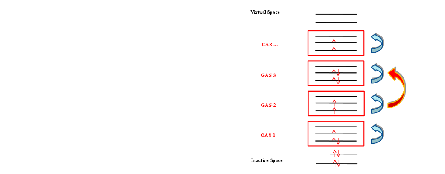
GASScf

Needed to perform a Generalized Active Space (GASSCF) calculation. It is followed by an integer that defines the number of active subspaces, and two lines for each subspace. The first line gives the number of orbitals in each symmetry, the second gives the minimum and maximum number of electrons in the accumulated active space.

An example of an input that uses this keyword is the following:

GASSCF 5 2 0 0 0 2 0 0 0 4 4 0 2 0 0 0 2 0 0 8 8 0 0 2 0 0 0 2 0 12 12 0 0 0 1 0 0 0 1 14 14 4 2 2 1 4 2 2 1 20 20

In the example above (20in32), excitations from one subspace to another are not allowed since the values of MIN and MAX for GSOC are identical for each of the five subspaces.

KSDFT Needed to perform MC-PDFT calculations. It must be used together with CIONLY keyword (it is a post-SCF method not compatible with SCF) and ROKS keyword. The functional choice follows. Currently available functionals are: tPBE, tBLYP, tLSDA. An example of an input that uses this keyword follows:
&RASSCF JOBIPH CIRESTART CIONLY Ras2 1 0 0 0 1 0 0 0 KSDFT ROKS TPBE In the above example, JOBIPH is used to use orbitals stored in JobIph, CIRESTART is used to use a pre-optimized CI vector, CIONLY is used to avoid conflicts between the standard RASSCF module and the MC-PDFT method (not compatible with SCF so far). The functional chosen is the translated–PBE.

JOBIph Input molecular orbitals are read from an unformatted file with FORTRAN file name JOBOLD. Note, the keywords Lumorb, Core, and Jobiph are mutually exclusive. If none is given the program will search for input orbitals on the runfile in the order: RASSCF, SCF, GUESSORB. If none is found, the keyword CORE will be activated.

IPHName Override the default choice of name of the JOBIPH file by giving the file name you want. The name will be truncated to 8 characters and converted to uppercase.

LUMOrb Input molecular orbitals are read from a formatted file with FORTRAN file name INPORB. Note, the keywords Lumorb, Core, and Jobiph are mutually exclusive. If none is given the program will search for input orbitals on the runfile in the order: RASSCF, SCF, GUESSORB. If none is found, the keyword CORE will be activated.

FILEorb Override the default name (INPORB) for starting orbital file by giving the file name you want.

CORE Input molecular orbitals are obtained by diagonalizing the core Hamiltonian. This option is only recommended in simple cases. It often leads to divergence. Note, the keywords Lumorb, Core, and Jobiph are mutually exclusive.

ALPHaOrBeta With UHF orbitals as input, select alpha or beta as starting orbitals. A positive value selects alpha, a negative value selects beta. Default is 0, which fails with UHF orbitals. This keyword does not affect the spin of the wave function (see the SPIN keyword).

TYPEIndex

This keyword forces the program to use information about subspaces from the INPORB file.

User can change the order of orbitals by editing of "Type Index" section in the INPORB file. The legend of the types is:

F - Frozen
I - Inactive
1 - RAS1
2 - RAS2
3 - RAS3
S - Secondary
D - Deleted

ALTEr This keyword is used to change the ordering of MO in INPORB or JOBOLD. The keyword requires first the number of pairs to be interchanged, followed, for each pair, the symmetry species of the pair and the indices of the two permuting MOs. Here is an example:
ALTEr= 2; 1 4 5; 3 6 8 In this example, 2 pairs of MO will be exchanged: 4 and 5 in symmetry 1 and 6 and 8 in symmetry 3.

CLEAnup This input is used to set to zero specific coefficients of the input orbitals. It is of value, for example, when the actual symmetry is higher than given by input and the trial orbitals are contaminated by lower symmetry mixing. The input requires at least one line per symmetry specifying the number of additional groups of orbitals to clean. For each group of orbitals within the symmetry, three lines follow. The first line indicates the number of considered orbitals and the specific number of the orbital (within the symmetry) in the set of input orbitals. Note the input lines can not be longer than 72 characters and the program expects as many continuation lines as are needed. The second line indicates the number of coefficients belonging to the prior orbitals which are going to be set to zero and which coefficients. The third line indicates the number of the coefficients of all the complementary orbitals of the symmetry which are going to be set to zero and which are these coefficients. Here is an example of what an input would look like:
CLEAnup 2 3 4 7 9; 3 10 11 13; 4 12 15 16 17 2 8 11; 1 15; 0 0; 0; 0 In this example the first entry indicates that two groups of orbitals are specified in the first symmetry. The first item of the following entry indicates that there are three orbitals considered (4, 7, and 9). The first item of the following entry indicates that there are three coefficients of the orbitals 4, 7, and 9 to be set to zero, coefficients 10, 11, and 13. The first item of the following entry indicates that there are four coefficients (12, 15, 16, and 17) which will be zero in all the remaining orbitals of the symmetry. For the second group of the first symmetry orbitals 8 and 11 will have their coefficient 15 set to zero, while nothing will be applied in the remaining orbitals. If a geometry optimization is performed the keyword is inactive after the first structure iteration.

CIREstart Starting CI-coefficients are read from a binary file JOBOLD.

ORBOnly This input keyword is used to get a formated ASCII file (RASORB, RASORB.2, etc) containing molecular orbitals and occupations reading from a binary JobIph file. The program will not perform any other operation. (In this usage, the program can be run without any files, except the JOBIPH file).

CIONly This keyword is used to disable orbital optimization, that is, the CI roots are computed only for a given set of input orbitals.

CHOInput

This marks the start of an input section for modifying the default settings of the Cholesky RASSCF. Below follows a description of the associated options. The options may be given in any order, and they are all optional except for ENDChoinput which marks the end of the CHOInput section.

NoLK Available only within ChoInput. Deactivates the ``Local Exchange'' (LK) screening algorithm [87] in computing the Fock matrix. The loss of speed compared to the default algorithm can be substantial, especially for electron-rich systems. Default is to use LK.

DMPK Available only within ChoInput. Modifies the thresholds used in the LK screening. The keyword takes as argument a (double precision) floating point (non-negative) number used as correction factor for the LK screening thresholds. The default value is 1.0d-1. A smaller value results in a slower but more accurate calculation.
Note.: The default choice of the LK screening thresholds is tailored to achieve as much as possible an accuracy of the converged RASSCF energies consistent with the choice of the Cholesky decomposition threshold.

NODEcomposition Available only within ChoInput. Deactivates the Cholesky decomposition of the inactive AO 1-particle density matrix. The inactive Exchange contribution to the Fock matrix is therefore computed using inactive canonical orbitals instead of (localized) ``Cholesky MOs'' [65]. This choice tends to lower the performances of the LK screening. Default is to perform this decomposition in order to obtain the Cholesky MOs.

TIME Activates printing of the timings of each task of the Fock matrix build. Default is to not show these timings.

MEMFraction Set the fraction of memory to use as global Cholesky vector buffer. Default: for serial runs 0.0d0; for parallel runs 0.3d0.

OFEMbedding Performs a Orbital-Free Embedding (OFE)RASSCF calculation, available only in combination with Cholesky or RI integral representation. The runfile of the environment subsystem renamed AUXRFIL is required. An example of input for the keyword OFEM is the following:
OFEMbedding ldtf/pbe dFMD 1.0 1.0d2 FTHAw 1.0d-4 The keyword OFEM requires the specification of two functionals in the form fun1/fun2, where fun1 is the functional used for the Kinetic Energy (available functionals: Thomas-Fermi, with acronym LDTF, and the NDSD functional), and where fun2 is the xc-functional (LDA, LDA5, PBE and BLYP available at the moment). The OPTIONAL keyword dFMD has two arguments: first, the fraction of correlation potential to be added to the OFE potential; second, the exponential decay factor for this correction (used in PES calculations). The OPTIONAL keyword dFMD specifies the fraction of correlation potential to be added to the OFE potential. The OPTIONAL keyword FTHA is used in a freeze-and-thaw cycle (EMIL Do While) to specify the (subsystems) energy convergence threshold.

ITERations Specify the maximum number of RASSCF iterations, and the maximum number of iterations used in the orbital optimization (super-CI) section. Default and maximum values are 200,100.

LEVShft Define a level shift value for the super-CI Hamiltonian. Typical values are in the range 0.0 – 1.5. Increase this value if a calculation diverges. The default value 0.5, is normally the best choice when Quasi-Newton is performed.

THRS Specify convergence thresholds for: energy, orbital rotation matrix, and energy gradient. Default values are: 1.0e-08, 1.0e-04, 1.0e-04.

TIGHt Convergence thresholds for the Davidson diagonalization procedure. Two numbers should be given: THREN and THFACT. THREN specifies the energy threshold in the first iteration. THFACT is used to compute the threshold in subsequent iterations as THFACT*DE, where DE is the RASSCF energy change. Default values are 1.0d-04 and 1.0d-3.

NOQUne This input keyword is used to switch off the Quasi-Newton update procedure for the Hessian. Pure super-CI iterations will be performed. (Default setting: QN update is used unless the calculation involves numerically integrated DFT contributions.)

QUNE This input keyword is used to switch on the Quasi-Newton update procedure for the Hessian. (Default setting: QN update is used unless the calculation involves numerically integrated DFT contributions.)

CIMX Specify the maximum number of iterations allowed in the CI procedure. Default is 100 with maximum value 200.

HEXS Highly excited states. Will eliminate the maximum occupation in one or more RAS/GAS's thereby eliminating all roots below. Very helpful for core excitations where the ground-state input can be used to eliminate unwanted roots. Works with RASSI. First input is the number of RAS/GAS where the maximum occupation should be eliminated. Second is the RAS/GAS or RAS/GAS's where maximum occupation will not be allowed.

SDAV Here follows the dimension of the explicit Hamiltonian used to speed up the Davidson CI iteration process. An explicit H matrix is constructed for those configurations that have the lowest diagonal elements. This H-matrix is used instead of the corresponding diagonal elements in the Davidson update vector construction. The result is a large saving in the number if CI iterations needed. Default value is the smallest of 100 and the number of configurations. Increase this value if there is problems converging to the right roots.

SXDAmp A variable called SXDAMP regulates the size of the orbital rotations. Use keyword SXDAmp and enter a real number. The default value is 0.0002. Larger values can give slow convergence, very low values may give problems e.g. if some active occupations are very close to 0 or 2.

SUPSym This input is used to restrict possible orbital rotations. It is of value, for example, when the actual symmetry is higher than given by input. Each orbital is given a label IXSYM(I). If two orbitals in the same symmetry have different labels they will not be allowed to rotate into each other and thus prevents from obtaining symmetry broken solutions. Note, however, that the starting orbitals must have the right symmetry. The input requires one or more entries per symmetry. The first specifies the number of additional subgroups in this symmetry ( a 0 (zero) denotes that there is no additional subgroups and the value of IXSYM will be 0 (zero) for all orbitals in that symmetry ). If the number of additional subgroups is not zero there are additional entries for each subgroup: The dimension of the subgroup and the list of orbitals in the subgroup counted relative to the first orbital in this symmetry. Note, the input lines can not be longer than 180 characters and the program expects continuation lines as many as there are needed. As an example assume an atom treated in C_2v symmetry for which the d_z² orbitals (7 and 10) in symmetries 1 may mix with the s orbitals. In addition, the d_z² and d_x²-y² orbitals (8 and 11) may also mix. Then the input would look like:
SUPSym 2 2 7 10; 2 8 11 0; 0; 0 In this example the first entry indicates that we would like to specify two additional subgroups in the first symmetry (total symmetric group). The first item in the following two entries declares that each subgroup consists of two orbitals. Orbitals 7 and 10 constitute the first group and it is assumed that these are orbitals of d_z² character. The second group includes the d_x²-y² orbitals 8 and 11. The following three entries denote that there are no further subgroups defined for the remaining symmetries. Ordering of the orbitals according to energy is deactivated when using SUPSym. If you activate ordering using ORDEr, the new labels will be printed in the output section. If a geometry optimization is performed the reordered matrix will be stored in the RUNFILE file and read from there instead of from the input in each new structure iteration.

HOME With this keyword, the root selection in the Super-CI orbital update is by maximum overlap rather than lowest energy.

IVO The RASSCF program will diagonalize the core Hamiltonian in the space of virtual orbitals, before printing them in the output. The resulting orbitals are only suitable to select which one should enter the active space in a subsequent calculation. The RASSCF calculation is not suitable for CASPT2/MRCI or any other correlated methods, becasue the energies of the virtual orbitals is undefined. This keyword is equivalent to IVO keyword of the SCF program.

VB Using this keyword, the CI optimization step in the RASSCF program will be replaced by a call to the CASVB program, such that fully variational valence bond calculations may be carried out. The VB keyword can be followed by any of the directives described in section and should be terminated by ENDVB. Energy-based optimization of the VB parameters is the default, and the output level for the main CASVB iterations is reduced to -1, unless the print level for CASVB print option 6 is $\geq$ 2.

The keyword is followed by a line giving the print levels for various logical code sections. It has the following structure: IW IPR IPRSEC(I), I=1,7

IW - logical unit number of printed output (normally 6).
IPR - is the overall print level (normally 2).
IPRSEC(I) - gives print levels in different sections of the program.
1. Input section
2. Transformation section
3. CI section
4. Super-CI section
5. Not used
6. Output section
7. Population analysis section

The meaning of the numbers: 0=Silent, 1=Terse, 2=Normal, 3=Verbose, 4=Debug, and 5=Insane. If input is not given, the default (normally=2) is determined by a global setting which can be altered bubroutine call. (Programmers: See programming guide). The local print level in any section is the maximum of the IPRGLB and IPRSEC() setting, and is automatically reduced e.g. during structure optimizations or numerical differentiation. Example:
Print= 6 2 2 2 3 2 2 2 2

MAXOrb Maximum number of RasOrb files to produce, one for each root up to the maximum.

OUTOrbitals

This keyword is used to select the type of orbitals to be written in a formated ASCII file. By default a formated RASORB file containing average orbitals and subsequent RASORB.1, RASORB.2, etc, files containing natural orbitals for each of the computed (up to ten) roots will be generated in the working directory. An entry follows with an additional keyword selecting the orbital type. The possibilities are:

AVERage orbitals: this is the default option. This keyword is used to produce a formated ASCII file of orbitals (RASORB) which correspond to the final state average density matrix obtained by the RASSCF program. The inactive and secondary orbitals have been transformed to make an effective Fock matrix diagonal. Corresponding diagonal elements are given as orbital energies in the RASSCF output listing. The active orbitals have been obtained by diagonalizing the sub-blocks of the average density matrix corresponding to the three different RAS orbital spaces, thereby the name pseudo-natural orbitals. They will be true natural orbitals only for a CASSCF wave function.

CANOnical orbitals: Use this keyword to produce the canonical orbitals. They differ from the natural orbitals, because also the active part of the Fock matrix is diagonalized. Note that the density matrix is no longer diagonal and the CI coefficients have not been transformed to this basis. This option substitutes the previous keyword CANOnical.

NATUral orbitals: Use this keyword to produce the true natural orbitals. The keyword should be followed by a new line with an integer specifying the maximum CI root for which the orbitals and occupation numbers are needed. One file for each root will be generated up to the specified number. In a one state RASSCF calculation this number is always 1, but if an average calculation has been performed, the NO's can be obtained for all the states included in the energy averaging. Note that the natural orbitals main use is as input for property calculations using SEWARD. The files will be named RASORB, RASORB.2, RASORB.3, etc. This keyword is on by default for up to ten roots.

SPIN orbitals. This keyword is used to produce a set of spin orbitals and is followed by a new line with an integer specifying the maximum CI root for which the orbitals and occupation numbers are needed. One file for each root will be generated up to the specified number. Note, for convenience the doubly occupied and secondary orbitals have been added to these sets with occupation numbers 0 (zero). The main use of these orbitals is to act as input to property calculations and for graphical presentations. This keyword is on by default for up to ten roots.

An example input follows in which five files are requested containing natural orbitals for roots one to five of a RASSCF calculation. The files are named RASORB.1, RASORB.2, RASORB.3, RASORB.4, and RASORB.5, respectively for each one of the roots. Although this is the default, it can be used complemented by the ORBOnly keyword, and the orbitals will be read from a JobIph file from a previous calculation, in case the formated files were lost or you require more than ten roots. As an option the MAXOrb can be also used to increase the number of files over ten.
OUTOrbital= Natural; 15

ORBListing

This keyword is followed with a word showing how extensive you want the orbital listing to be in the printed output. The alternatives are:

NOTHing: No orbitals will be printed (suggested for numerical CASPT2 optimization). (Also, the old VERYbrief will be accepted).
FEW: The program will print the occupied orbitals, and any secondary with less than 0.15 a.u. orbital energy. (Old BRIEF also accepted).
NOCOre: The program will print the active orbitals, and any secondary with less than 0.15 a.u. orbital energy.
ALL: All orbitals are printed. (Old LONG also accepted).

(unless other limits are specified by the PROR keyword).

ORBAppear

This keyword requires an entry with a word showing the appearance of the orbital listing in the printed output. The alternatives are:

COMPact: The format of the orbital output is changed from a tabular form to a list giving the orbital indices and MO-coefficients. Coefficients smaller than 0.1 will be omitted.
FULL: The tabular form will be chosen.

PROR This keyword is used to alter the printout of the MO-coefficients. Two numbers must be given of which the first is an upper boundary for the orbital energies and the second is a lower boundary for the occupation numbers. Orbitals with energy higher than the threshold or occupation numbers lower that the threshold will not be printed. By default these values are set such that all occupied orbitals are printed, and virtual orbitals with energy less than 0.15 au. However, the values are also affected by use of OUTPUT.

PRSD This keyword is used to request that not only CSFs are printed with the CI coefficients, but also the determinant expansion.

ORDEr This input keyword is used to deactivate or activate ordering of the output orbitals according to energy. One number must be given: 1 if you want ordering and 0 if you want to deactivate ordering. Default is 1 and with SUPSym keyword default is 0.

PRSP Use this keyword to get the spin density matrix for the active orbitals printed.

PRWF Enter the threshold for CI coefficients to be printed (Default: 0.05).

TDM If this keyword is given, and if HDF5 support is enabled, the active 1-electron transition density matrix between every pair of states in the current calculation will be computed and stored in the HDF5 file.

DMRG Specify maximum number of renormalized states (or virtual bond dimension m) in each microiteration in DMRG calculations. m must be integer and should be at least 500. This keyword is supported in both CheMPS2 and Block interfaces. Note that DMRG-CASSCF calculations for excited states are not fully supported by the Block interface.

3RDM Use this keyword to get the 3-particle and Fock matrix contracted with the 4-particle reduced density matrices (3-RDM and F.4-RDM) for DMRG-CASPT2. OUTOrbitals = CANOnical is automatically activated. In CheMPS2 interface, both 3-RDM and F.4-RDM are calculated. In Block interface, only 3-RDM is calculated while F.4-RDM is approximated in the CASPT2 module.

CHBLb Specify a threshold for activating restart in CheMPS2. After each macroiteration, if the max BLB value is smaller than CHBLb, activate partial restart in CheMPS2. If the max BLB value is smaller than CHBLb/10.0, activate full restart in CheMPS2. Default value is: 0.5d-2.

DAVTolerance Specify value for Davidson tolerance in CheMPS2. Default value is 1.0d-7.

NOISe Specify value for noise pre-factor in CheMPS2. This noise is set to 0.0 in the last instruction. Default value (recommended) is: 0.05

MXSWeep Maximum number of sweeps in the last instruction in CheMPS2. Default value is: 8. In the last iteration of DMRG-SCF, MXSW is increased by five times (default 40).

MXCAnonical Maximum number of sweeps in the last instruction with pseudocanonical orbitals in CheMPS2. Default value is: 40.

CHREstart Use this keyword to activate restart in the first DMRG iteration from a previous calculation. The working directory must contain molcas_natorb_fiedler.txt and CheMPS2_natorb_MPSx.h5 (x=0 for the ground state, 1 for the first excited state, etc). If these files are not in the working directory, a warning is printed at the beginning of the calculation and restart is skipped (start from scratch).

DMREstart

Use this keyword to activate restart in the last DMRG iteration from the previous iteration or calculation. This keyword only works when using OUTOrbitals = CANOnical or 3RDM.

DMREstart = 0 (default): start from scratch to calculate 3-RDM and F.4-RDM.

DMREstart = 1: start form user-supplied checkpoint files. The working directory must contain molcas_canorb_fiedler.txt and CheMPS2_canorb_MPSx.h5 (x=0 for the ground state, 1 for the first excited state, etc). If these files are not in the working directory, a warning is printed at the beginning of the calculation and restart is skipped (start from scratch).

DMREstart = 2 (Not recommended): start form previous checkpoint files with natural orbitals. DMREstart = 2 is not recommended since this may produce non-optimal energy because the orbital ordering is not optimized.

A general comment concerning the input orbitals: The orbitals are ordered by symmetry. Within each symmetry block the order is assumed to be: frozen, inactive, active, external (secondary), and deleted. Note that if the Spdelete option has been used in a preceding SCF calculation, the deleted orbitals will automatically be placed as the last ones in each symmetry block.

For calculations of a molecule in a reaction field see section

of the present manual and section

of the examples manual.

8.41.5.2 Input example

The following example shows the input to the RASSCF program for a calculation on the water molecule. The calculation is performed in C_2v symmetry (symmetries: a₁, b₂, b₁, a₂, where the two last species are antisymmetric with respect to the molecular plane). Inactive orbitals are 1a₁ (oxygen 1s) 2a₁ (oxygen 2s) and 1b₁ (the $\pi$ lone-pair orbital). Two bonding and two anti-bonding OH orbitals are active, a₁ and b₂ symmetries. The calculation is performed for the ¹A₁ ground state. Note that no information about basis set, geometry, etc has to be given. Such information is supplied by the SEWARD integral program via the one-electron integral file ONEINT.

&RASSCF Title= Water molecule. Active orbitals OH and OH* in both symmetries Spin = 1 Symmetry = 1 Inactive = 2 0 1 0 Ras2 = 2 2 0 0

The following input is an example of how to use the RASSCF program to run MC-PDFT calculations:
&RASSCF Ras2 1 0 0 0 1 0 0 0 >>COPY $CurrDir/$Project.JobIph JOBOLD &RASSCF JOBIPH CIRESTART CIONLY Ras2 1 0 0 0 1 0 0 0 KSDFT ROKS TPBE The first RASSCF run is a standard CASSCF calculation that leads to variationally optimized orbitals and CI coefficients. The second call to the RASSCF input will use the CI vector and the orbitals previously optimized. The second RASSCF will require the CIONLY keyword as the MC-PDFT is currently not compatible with SCF. KSDFT ROKS and the functional choice will provide MC-PDFT energies.

&RASSCF Title= Water molecule. Active orbitals OH and OH* in both symmetries Spin = 1 Symmetry = 1 Inactive = 2 0 1 0 Ras2 = 2 2 0 0 DMRG = 500 3RDM